1 Introduction

There are three kinds of lies: lies, damned lies, and statistics.

Anonymous, but popularized by Mark Twain.

SEATTLE Local News – Two Seconds Cost $74 Million.¹

¹ $74 million later, Mercer Mess is 2 seconds faster, KOMO News 2016; case from callingbullshit.

That amount was set aside to improve the Mercer Mess. Lanes were added. Signal capacity was improved.

Now GPS navigator TomTom, which tracks drivers using its app, says the average time through the corridor during the peak morning commute 7 minutes, 50 seconds before the Mercer Mess construction.

And now the travel time through Mercer is 7 minutes and 48 seconds. That’s right. An improvement of 2 seconds.

1.1 Introduction

1.1.1 Teaching Staff Introduction

Instructor: Haoyu Yue | [email protected]

Office Hours: 9:20-10:20 AM on Monday at Gould Hall 012C; or online by appointment

Teaching assistant: Sun Ho Hwang | [email protected]

Office Hours: 10:00-11:00 AM on Friday at Gould Hall 432 (Urban Ecology lab)

1.1.2 Pre-class Survey

35 out of 47 students answered the pre-class survey before the end of September 30.

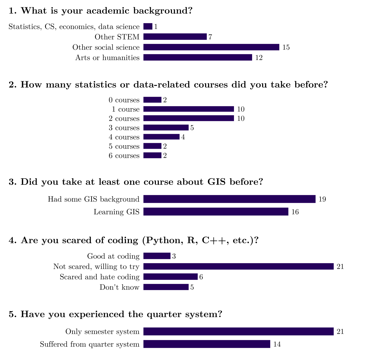
Figure 1.1: Answers to the pre-class survey, 35 responses. Answers are shortened.

And we received some comments:

Very excited
Excited to learn such hard skills
Learned R in an intense way and love to learn more R
Learned R in an intense way and think it is beneficial
Like an expert in informatics and data science
Wish to better use R
Took some data science classes
Nervous but looking forward to it
Used R before but cannot remember anything
Bad at math and coding
Very scared

1.1.3 Self-Introduction

For example:

Your name and pronouns
Your affiliation and year in the program
The reason you pursue a master degree in urban planning
Your experience/interests with statistics, coding, and quantitative data
Your expectations for this class
Recent happiness (accomplishment, hobby, adventure, etc.)

1.1.4 Course Overview

Planning has always been built on the facts we observed, the future we anticipated, the good scenarios we wished for, and the correct interventions we relied on. But are the facts really facts? Will that future actually arrive? Is a number a good way to define the good? And are the correct interventions actually correct?

Quantitative Methods is a core course for Master of Urban Planning students at the University of Washington. It intends to serve as a foundation for taking on these questions with data, and a stepping stone toward advanced quantitative methods in the broader social sciences. We will work together this quarter, 6 hours per week, starting from where every number begins and spending the quarter making numbers, doubting them, connecting them, and deciding with them. You may not leave with an answer, but you will certainly carry away questions worth asking.

1.2 Way of Knowing

Epistemology is a branch of philosophy, which is about the theory of knowledge. For example, they ask how we know what we know and what we can regard as acceptable knowledge.

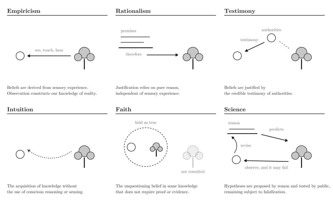
Figure 1.2: Some ways of knowing: How do we ‘know’ that this tree exists?

1.2.1 Research is a Process of Knowing

Science is a way of knowing while research is the process of finding out the answers, correct or incorrect. Or broadly speaking, research is a process that we gather information systematically to generate new insights and/or answer some problems. For example, we can have:

Problem: How many homeless individuals are living in King County?
Research: Count each homeless individual within King County one by one.

This research approach is obviously infeasible. But any other methodologies we use would be an estimation of the real count. Every decision researchers made would influence the final results. The King County Regional Homelessness Authority’s five-year plan (P.8) reports five different counts from five different agencies:

Measure	Lead agency	Individuals
2020 Point in Time Count	All Home	11,751
2022 Point in Time Count	KCRHA	13,368
2023 Snapshot Report	WA Department of Commerce	34,866
2020 Cross-Systems Analysis	King County Dept. of Community and Health Services	40,871
2022 Housing Gaps Analysis	WA Dept. of Commerce and Cloudburst Consulting	53,532

Table 1.1: Number of homeless individuals in King County based on different research

The largest is 4.6 times the smallest. We cannot say any of them is a mistake. Each answers a slightly different question. They are counts from different time windows, different definitions of homeless individuals, different data-collection machinery, and different methodologies.

However, as you can imagine, planners will make different decisions, or even opposite decisions if they just use numbers without thinking deeper about some critical questions. Research is not the pursuit of the number; it is the practice of making these choices reasonable and explicit, so that someone else can see what you did, then agree or disagree with it precisely.

1.2.2 Quantitative vs. Qualitative

Data is a collection of facts, numbers, words, observations, or other useful information. We can generally classify data by whether it can be measured/represented using numbers.

Data Types	Methods
Quantitative Data: values that can be measured numerically, such as population, housing prices.	Statistical modeling, simulations, etc.
Qualitative Data: descriptive and non-numerical, capturing characteristics, concepts, or experiences that numbers cannot measure, such as an interview transcript or a survey response.	Case study, text analysis, certain statistical methods, etc.

Table 1.2: Quantitative and qualitative data

1.2.3 Research Paradigms

However, quantitative or qualitative research refers more to the way we analyze data and approach the questions, rather than to the data alone. This taxonomy represents two paradigms of scientific discovery: positivist (associated more with quantitative methods) and constructionist (associated more with qualitative methods) (Gliner et al. 2017).

Gliner, Jeffrey A., George A. Morgan, and Nancy L. Leech. 2017. Research Methods in Applied Settings: An Integrated Approach to Design and Analysis. Third edition. Routledge, Taylor & Francis Group.

Paradigm	Positivist	Constructionist
The nature of reality	Single reality	Multiple constructed realities
Relationship of knower to known	Researchers are objective	Researchers cannot be totally objective; in fact, researchers and participants interact
Possibility of generalization	Could be generalized	Everything is contextually bound
Possibility of causal linkage	Could at least partially determined	Cannot distinguish cause and effect
The role of value	Research is objective and value free	Bound by choice, values, theory, and conflict

Table 1.3: Positivist and constructionist paradigm

Not all quantitative research is purely positivist, and qualitative research is constructionist. This table reflects the relative differences, and we normally find that most research in planning is a mix of the two. Also, you may realize that quantitative research could use qualitative data (e.g., encoding an interview scripts to find statistical relationship), which we call mixed method. This class is focusing on quantitative analysis and URBAN 518 (Autumn quarter 2nd year of MUP) will focus on qualitative analysis.

1.3 Math Review

1.3.1 Order of Operations

Evaluate an expression in this order: parentheses, exponents, multiplication and division, then addition and subtraction. Multiplication and division rank equally and are worked left to right, as are addition and subtraction. \[4^3 \times 3^2 - 10 + 27/3 \;=\; 64 \times 9 - 10 + 9 \;=\; 575\]

1.3.2 Fractions

A fraction is a numerator over a denominator. To multiply, multiply numerators and denominators separately; to divide, multiply by the reciprocal: \[\frac{1}{2} \times \frac{3}{4} = \frac{1 \times 3}{2 \times 4} = \frac{3}{8}, \quad \frac{1}{2} \div \frac{3}{4} = \frac{1}{2} \times \frac{4}{3} = \frac{2}{3}\]

Adding or subtracting requires a common denominator: $\frac{1}{3} + \frac{1}{4} = \frac{4}{12} + \frac{3}{12} = \frac{7}{12}$.

Every rate is a fraction, and every unit conversion is a fraction multiplication: one-third of an acre per 100 people is $\frac{1/3}{100} \times 1000 = 3.33$ acres per 1,000 people.

1.3.3 Solving for an Unknown

Apply the same operation to both sides of an equation until the unknown stands alone. Both sides stay equal because each received the same change. A standard of 8 acres per 1,000 residents, at a projected population of 806,800, requires $a$ acres: \[\frac{a}{806{,}800} \times 1000 = 8 \;\Longrightarrow\; a \times 1000 = 8 \times 806{,}800 \;\Longrightarrow\; a = \frac{8 \times 806{,}800}{1000} = 6{,}454.4\]

1.3.4 Lines and Slope

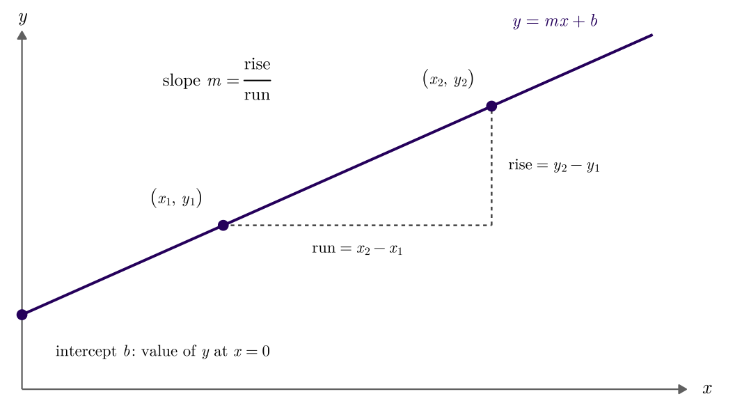
A line is written $y = mx + b$. The slope $m$ is the change in $y$ per one-unit change in $x$; the intercept $b$ is the value of $y$ when $x = 0$. Given two points $(x_1, y_1)$ and $(x_2, y_2)$: \[m = \frac{y_2 - y_1}{x_2 - x_1}, \qquad b = y_1 - m x_1\]

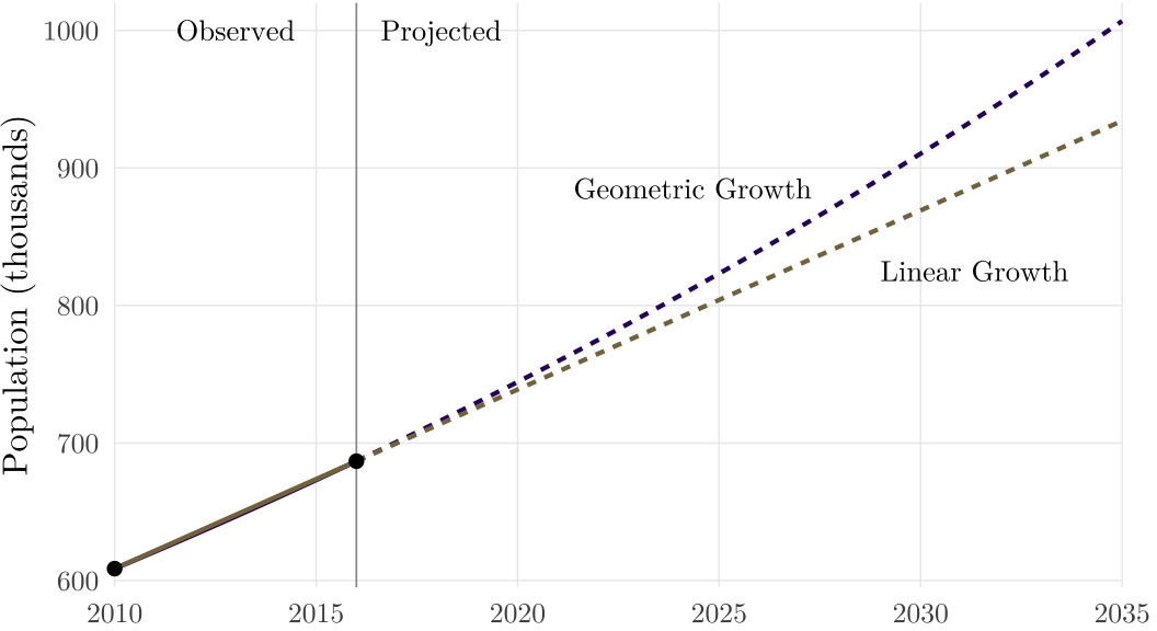
The slope is the rise over the run, and its sign says whether $y$ increases or decreases as $x$ increases. Seattle’s population was 608,660 in 2010 and 686,800 in 2016, so the slope through those two points is $(686{,}800 - 608{,}660) / (2016 - 2010) \approx 13{,}023$ people per year: the average annual increment implied by a straight line.

Figure 1.3: Anatomy of a line. The slope is the rise over the run; the intercept is the height of the line at $x=0$.

1.3.5 Percent versus Percentage Point

A percentage point is an arithmetic difference between two percentages. A percent change is a relative change. Moving from 20% to 25% is a rise of 5 percentage points and a rise of 25 percent.

The Seattle Parks and Open Space Plan contains the sentence that:

about 23% of Seattleites are aged 25 to 34, “which is up 21% from 2010”.

This is a relative increase in the count, not a shift of 21 percentage points in the share. Read the wrong way, that sentence implies a 2010 share of 2%.

1.3.6 Growth Rates

Given a starting value $P_0$ and an ending value $P_1$ separated by $n$ years, the compound annual growth rate (CAGR) is the constant yearly rate that would carry one to the other: \[\text{CAGR} = \sqrt[n]{\frac{P_1}{P_0}} - 1 = \left(\frac{P_1}{P_0}\right)^{1/n} - 1 \]

If projecting, a linear assumption adds a fixed number of people each year while a geometric assumption multiplies by a fixed factor. Over a twenty-year horizon, the two diverge substantially.

Figure 1.4: Linear and geometric growth through Seattle’s 2010 and 2016 populations (608,660 and 686,800). The linear path adds 13,023 people a year; the geometric path grows 2.03% a year, the CAGR.

1.3.7 Weighted Averages

The mean of a set of subgroup means is not the mean of the whole unless the subgroups are the same size. With groups of size $n_j$ and group means $\bar{y}_j$, the correct combination is

\[\bar{y} = \frac{n_1}{n}\,\bar{y}_1 + \frac{n_2}{n}\,\bar{y}_2 + \cdots + \frac{n_k}{n}\,\bar{y}_k , \quad n = n_1 + n_2 + \cdots + n_k\]

Example 1.1 Calculate the average age of two groups.

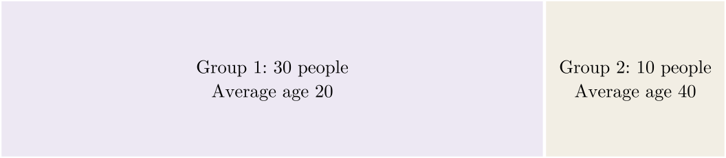
Figure 1.5: Two groups of 30 and 10 people and their average ages. Each group’s area is its share of the whole.

The overall average age needs to be weighted by the proportion of people, not simply the average of the two group averages.

\[\text{Overall Age} = \frac{30}{30+10} \times 20 + \frac{10}{30+10} \times 40 = 25\]

1.3.8 Notation and Calculus

1.3.8.1 Function

A function $f(x)$ assigns one output to each input. The domain is the set of allowed inputs; the range is the set of possible outputs.

For example, $f(x) = 2x + 1$ maps the input $x = 3$ to the output $f(3) = 2 \times 3 + 1 = 7$. Its domain and range are all real numbers. The function $g(x) = 1/x$ is undefined at $x = 0$, so its domain is every $x \ne 0$.

1.3.8.2 Summation

$\sum_{i=1}^{n} x_i = x_1 + x_2 + \cdots + x_n$. The index $i$ runs over the cases; $n$ is the number of cases.

Note that $\sum x_i^2$ and $\left(\sum x_i\right)^2$ are different: for the values 1, 2, 3, $\sum x_i^2 = 14$ while $\left(\sum x_i\right)^2 = 36$.

1.3.8.3 Factorial

$n! = n(n-1)(n-2)\cdots 1$, with $0! = 1$. Example: $4! = 4 \times 3 \times 2 \times 1 = 24$. Appears in counting formulas for arrangements and combinations.

Why 0! = 1.

Based on the definition, we can know the factorial in terms of the next one:

\[n! = \frac{(n+1)!}{n+1}\]

So that

\[0! = \frac{(0+1)!}{0+1} = \frac{1!}{1} = \frac{1}{1} = 1\]

Defining 0! = 1 is the only way to keep this mathematical logic consistent.

1.3.8.4 Exponents and Roots

$a^n$ means $a$ multiplied by itself $n$ times; $a$ is the base and $n$ the exponent. Exponents need not be whole numbers. \[a^m a^n = a^{m+n}, \quad (a^m)^n = a^{mn}, \quad \frac{a^m}{a^n} = a^{m-n}, \quad a^{-n} = \frac{1}{a^n}, \quad a^0 = 1\]

A root is a fractional exponent: $a^{1/2} = \sqrt{a}$, and $a^{1/n}$ is the $n$th root of $a$.

1.3.8.5 Logarithm

The inverse of exponentiation: if $y = a^x$, then $\log_a y = x$.

Some rules: $\log(xy) = \log x + \log y$; $\log(x/y) = \log x - \log y$; $\log(x^k) = k \log x$.

In these notes $\log$ denotes the natural logarithm, base $e \approx 2.718$, with inverse $\exp(x) = e^x$.

Reference: What’s so special about Euler’s number e? 3Blue1Brown

1.3.8.6 Limit

$\lim_{x \to a} f(x) = L$: the value of $f(x)$ can be made close to $L$ by taking $x$ close enough to $a$, with $x \ne a$. The target $a$ is a number or $\pm\infty$, and “close enough” reads differently in each case:

$x \to \infty$: $x$ large enough. Written $\lim_{n \to \infty}$, it underlies “as $n$ grows” statements.
$x \to -\infty$: $x$ negative enough.
$x \to a$ for a number $a$: $|x - a|$ small enough. The derivative below takes $h \to 0$, that is, $|h|$ small enough.

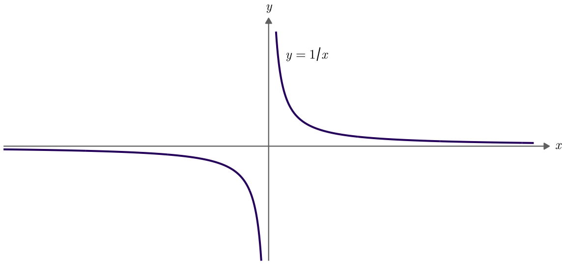
For $f(x) = 1/x$, $\lim_{x \to \infty} 1/x = 0$ and $\lim_{x \to -\infty} 1/x = 0$ (Figure 1.6). The limit is the value approached, not a value reached.

Figure 1.6: The limit of $1/x$ as $x \to \infty$ or $x \to -\infty$ is $0$.

1.3.8.7 Matrix

An $n \times k$ matrix is a rectangular array with $n$ rows and $k$ columns; a vector is a single column. A data frame is a matrix with named columns.

\[\mathbf{X} = \begin{bmatrix} x_{11} & x_{12} & \cdots & x_{1k} \\ x_{21} & x_{22} & \cdots & x_{2k} \\ \vdots & \vdots & \ddots & \vdots \\ x_{n1} & x_{n2} & \cdots & x_{nk} \end{bmatrix}, \qquad \mathbf{y} = \begin{bmatrix} y_1 \\ y_2 \\ \vdots \\ y_n \end{bmatrix}\]

The entry $x_{ij}$ sits in row $i$ and column $j$. In a data set, row $i$ is case $i$ and column $j$ is variable $j$. The vector $\mathbf{y}$ is $n \times 1$: one value per case.

1.3.8.8 Derivative

$f'(x) = \lim_{h \to 0} \frac{f(x+h) - f(x)}{h}$: the changing rate of $f$ at $x$, the slope of the tangent line at that point. Common rules:

$\frac{d}{dx} x^n = n x^{n-1}$
$\frac{d}{dx} e^x = e^x$
$\frac{d}{dx} \ln x = 1/x$
$[f(x)g(x)]' = f'(x)g(x) + f(x)g'(x)$ (product rule)
$[f(g(x))]' = f'(g(x))\, g'(x)$ (chain rule)

For $f(x) = x^2$ at $x = 1$, the line through $(1, 1)$ and $(1 + h, (1 + h)^2)$ has slope

\[\frac{(1 + h)^2 - 1^2}{h} = \frac{2h + h^2}{h} = 2 + h .\]

As $h \to 0$ the slope goes to $2$, which matches: $f'(1) = 2 \times 1 = 2$ (Figure 1.7).

Figure 1.7: The derivative of $f(x) = x^2$ at $x = 1$. Left: lines through $(1, 1)$ and $(1 + h, (1 + h)^2)$ have slope $2 + h$.

1.3.8.9 Integral

$\int_a^b f(x)\,dx$ is the area under $f$ between $a$ and $b$.

An antiderivative of $f$ is any $F$ with $F'(x) = f(x)$, written $\int f(x)\,dx = F(x) + C$; so that $\int_a^b f(x)\,dx = F(b) - F(a)$. Some basic forms:

$\int x^n\,dx = \frac{x^{n+1}}{n+1} + C$ for $n \ne -1$
$\int \frac{1}{x}\,dx = \ln|x| + C$
$\int e^x\,dx = e^x + C$

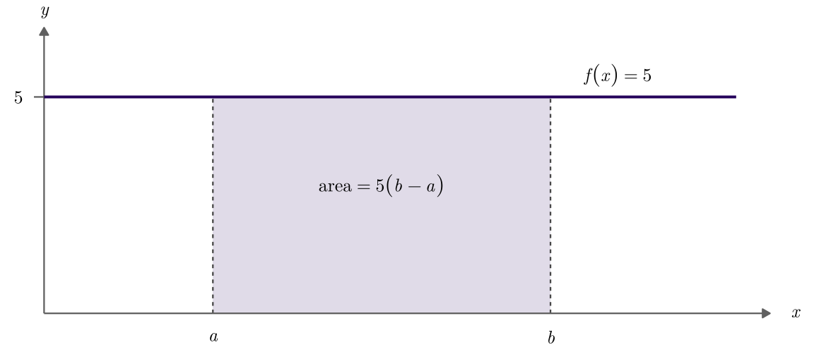
For the constant function $f(x) = 5$, the antiderivative $F(x) = 5x + C$ gives: $F(b) - F(a) = 5b - 5a$. In another way, the region under $f$ between $a$ and $b$ is a rectangle of height $5$ and width $b - a$ (Figure 1.8):

Figure 1.8: The integral of the constant function $f(x) = 5$ from $a$ to $b$ is the shaded rectangle, with area $5(b - a)$.

Example 1.2 Density and distribution function. For a variable $X$, we can define $F$ as the accumulated area below the curve from $-\infty$ to $x_o$ (an integral operation):

\[F(x_0) = \int_{-\infty}^{x_0} f(t)\,dt = P(X \le x_0)\]

Differentiating undoes the accumulation and returns the $f(x_0)$, which is a rate how fast $F$ is accruing at $x_0$:

\[f(x_0) = F'(x_0) = \lim_{h \to 0} \frac{F(x_0 + h) - F(x_0)}{h} .\]

Figure 1.9: Differentiation and integration are one relationship read in two directions. Integrating the density $f$ up to $x_0$ gives the area $F(x_0) = P(X \le x_0)$; differentiating $F$ at $x_0$ gives back the height $f(x_0)$, which is the slope.