2 Describing Numbers
Hear about the statistician who drowned crossing a river? It was three feet deep on average.
Anonymous
2.1 Levels of Measurement
Nominal scales are labels with no order, such as a ZIP code, a housing type code (1 = single family, 2 = townhouse, 3 = apartment), a land use category. Nominal categories cannot be rank-ordered. Only the mode, the most frequent value, summarizes them. The mean of a set of ZIP codes has no meaning.
Ordinal scales are ordered, but the gaps between adjacent categories are not equal: a design review outcome (pass, pass with conditions, fail), a level of satisfaction from 1 to 3, a hazard mitigation plan’s probability rating from 1 to 4. The median, the middle value once the cases are sorted, and the mode are meaningful. The mean is not: it treats the step from 1 to 2 as equal in size to the step from 4 to 5, and the scale does not guarantee that.
Example 2.1 The American Public Health Association’s 1945 Appraisal Method scored housing quality for urban renewal by assigning penalty points to each of 29 deficiency items, for example:
- 45 for lacking a toilet
- 30 for lacking dual egress
- 20 for obstructed daylight
- 3 for lacking central heating
Then, sum them to a dwelling total with a maximum of 600. The order of penalty points is reasonable: lacking a toilet is worse than obstructed daylight. The sum is not (Hodge 1963).
Interval scales have equal distances and an arbitrary zero. Temperature is the standard case: means are meaningful, ratios are not (80 degrees is not twice as hot as 40).
Ratio scales have equal distances and a true zero, such as commuting minutes, parcel area in square feet, dollars, acres. Every summary is available.
| Level | Planning example | Meaningful summaries |
|---|---|---|
| Nominal | ZIP code, land use class | mode |
| Ordinal | design review outcome | mode, median, percentiles |
| Interval | temperature in Fahrenheit | mode, median, mean, standard deviation |
| Ratio | acres, minutes, dollars | all of the above, plus ratios |
2.2 Population and Sample
A population is the entire group of people or things about which we want information. For example, all people lived in Seattle during 2026. However, it is more practical to gain information about the whole population by only examining a part. Sample is a smaller subset of a larger set of data to draw inferences about the large set, such as 1,000 selected people lived in Seattle during 2026.
We always are interested in some quantities of population, such as the average age. We call such quantity a parameter. The quantities we calculate from this sample are called statistics.
The process of collecting samples from population is sampling and the process of estimate parameter based on samples is inference.
It is important to first identify whether your data is “population” or “sample”. If it is the population, no inference is needed. Just descriptive analysis. If it is the sample, we need to consider how to collect the sample and the associated sampling errors and uncertainty.
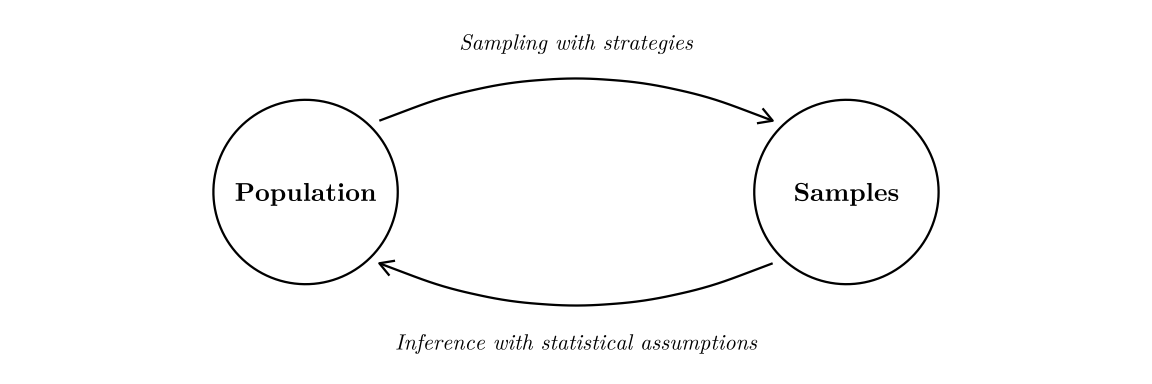
Example 2.2 Estimate the average age of people lived in Seattle during 2026.
- Population: all people living in Seattle during 2026
- Sample: 1,000 selected people who lived in Seattle during 2026
- Parameter: the true average age of people who lived in Seattle during 2026 (UNKNOWN unless we survey everybody)
- Statistic: the average age of 1,000 selected people who lived in Seattle during 2026
2.3 Frequency Table
A frequency table is a listing of possible values for a variable, together with the number of observations for each value. A proportion of observations that fall in a certain category is the count of observations in that category divided by the total number of observations. (NOTE: percent = 100 \(\times\) proportion)
| Mode of travel to work | Frequency | Proportion | Percent |
|---|---|---|---|
| Drove alone | 147 | 0.411 | 41.1% |
| Carpooled | 29 | 0.081 | 8.1% |
| Public transit | 86 | 0.240 | 24.0% |
| Walked | 43 | 0.120 | 12.0% |
| Bicycle | 15 | 0.042 | 4.2% |
| Taxi, motorcycle, or other | 8 | 0.022 | 2.2% |
| Worked at home | 30 | 0.084 | 8.4% |
| Total | 358 | 1.000 | 100.0% |
2.4 Measures of Center
The sample mean, written \(\bar{y}\) and read “y-bar”, is the total divided by the count. Average is a more general and everyday representation for the similar meaning.
\[\bar{y} \;=\; \frac{1}{n} \sum_{i=1}^{n} y_i\]
Percentiles is score below which a specific percentage of the distribution falls. For example, the 75th percentile is a score that divides the distribution so that 75% of the cases are below it.
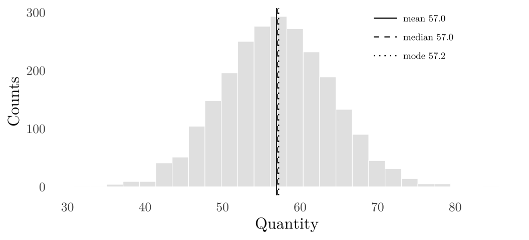
Median is 50th percentile. When \(n\) is even, median is the average of the middle two values. Mode is the value that appears most frequently. On a symmetric distribution mean, median, and mode nearly coincide.
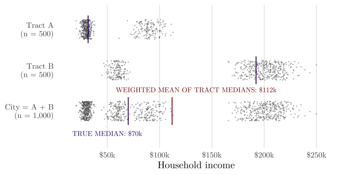
Example 2.3 Medians do not add: the averaging the medians of the parts does not give the median of the whole; the median is not an additive quantity. The arithmetic mean of census tract median household incomes is not the city’s median household income, and weighting each tract by its population does not repair it.
2.5 Measures of Spread
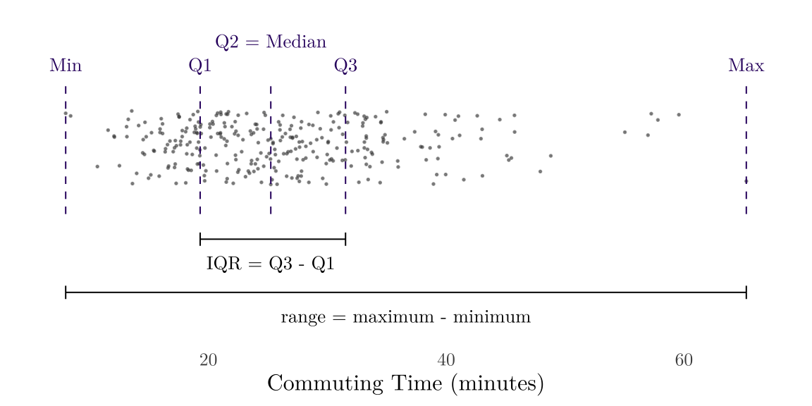
Minimum is the smallest value while maximum is the largest value. We use the difference between max and min to represent the range of data: Range = Maximum - Minimum.
After arranging the data from smallest to largest, the first quartile (Q1) is the 25th percentile of data, the second quartile (Q2) is the 50th percentile of data (which is the median), the third quartile (Q3) is the 75th percentile of data. The interquartile range (IQR) is the 75th percentile minus the 25th.
If we have every unit of a population, the population standard deviation (\(\sigma\)) measures how far a typical unit sits from the population mean \(\mu\): subtract \(\mu\) from each value, square the deviations, average them over the \(N\) units, and take the square root. Without the square root, the result is the population variance (\(\sigma^2\)).
\[\sigma \;=\; \sqrt{\frac{1}{N} \sum_{i=1}^{N} \left(y_i - \mu\right)^2}\]
Usually we only have a sample and we want to estimate the SD or variance from it. The sample standard deviation (\(s\)) estimates \(\sigma\) from the sample. Without the square root, the result is the sample variance (\(s^2\)), the estimate of \(\sigma^2\).
\[s \;=\; \sqrt{\frac{1}{n-1} \sum_{i=1}^{n} \left(y_i - \bar{y}\right)^2}\]
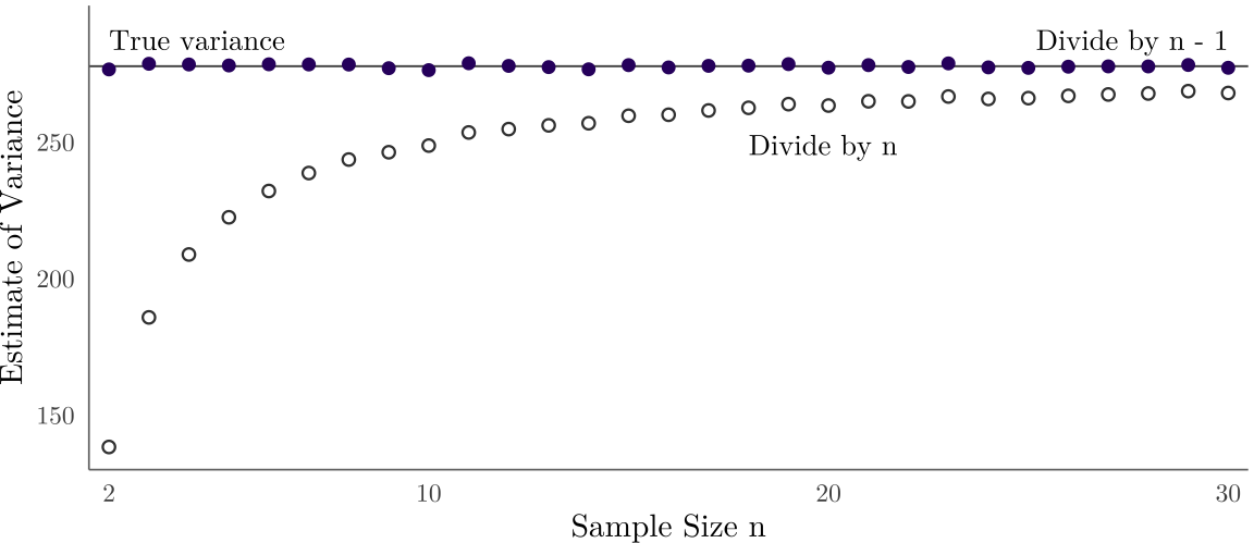
The divisor is \(n - 1\) rather than \(n\) because the deviations are measured from the sample’s own mean, which sits closer to the sample than population mean \(\mu\) and so understates the population’s spread.
Example 2.4 Some samples are drawn from a population whose true variance is known (horizontal line). Dividing the squared deviations (\(\sum_{i=1}^{n} \left(y_i - \bar{y}\right)^2\)) by \(n\) underestimates the true variance. The deviations are measured from the sample’s own mean, which sits closer to its own sample than the box mean does. Dividing by n - 1 corrects the bias.
2.5.1 Population and Sample Variance Proof
Let \(Y_1, Y_2, \dots, Y_n\) be a random sample of size \(n\) drawn from a population. The sample variance should be a unbiased estimator, which means \(E(s^2) = \sigma^2\) (expectation of sample variance should be equal to population variance).
Each \((y_i - \bar{y}) = (y_i - \mu) - (\bar{y} - \mu)\); so that: \(\sum_{i=1}^{n} (y_i - \bar{y})^2 \;=\; \sum_{i=1}^{n} (y_i - \mu)^2 \;-\; n\,(\bar{y} - \mu)^2\). We know the true variance \(\sigma^2\):
\[\begin{aligned} \sigma^2 &= \frac{1}{n}\,E\!\left[\sum_{i=1}^{n} (y_i - \mu)^2\right] \\ &= \frac{1}{n}\,E\!\left[\sum_{i=1}^{n} (y_i - \bar{y})^2 + n\,(\bar{y} - \mu)^2\right] \\ &= \frac{1}{n}\,E\!\left[\sum_{i=1}^{n} (y_i - \bar{y})^2\right] + \operatorname{Var}(\bar{y}) \\ &= \frac{1}{n}\,E\!\left[\sum_{i=1}^{n} (y_i - \bar{y})^2\right] + \frac{\sigma^2}{n} \\ (1-\frac 1n) \sigma^2 &= \frac{1}{n}\,E\!\left[\sum_{i=1}^{n} (y_i - \bar{y})^2\right] \\ \sigma^2 &= E\!\left[\frac 1 {n-1}\sum_{i=1}^{n} (y_i - \bar{y})^2\right] \end{aligned}\] We proof the sample variance should be divided by \(n-1\).
2.6 Measures of Shape
Figure 2.2 is a symmetric distribution. On a right-skewed distribution (one with a long tail of large values), the tail pulls the mean above the median, and the gap between the two reflects the length of the tail (Figure 2.7). Planning data are typically right-skewed: income, rent, parcel area, commuting time, house price. You can imagine what left-skewed means: one with a long tail of small values.
2.7 Some Dataset Formats
2.7.1 Tabular
The standard data formats is tabular data (a data frame): one row per record/item/observation/data point, one column per variable/feature/attribute.1 Even through there could be some missing cells but we have a fixed structure, we call those structured data. So, unstructured data lacks a predefined or organized data model, such as text, images, or videos. This course is mainly based on tabular data.
1 When processing data in R/Python, we should use machine-readable column names: median_rent, not Median Rent. Spaces in column names break many pipelines.
Based on the contents within a tabular data, we can classify by the shapes. For example, each cell below is a home-value index for a metro area in a month, with a population column appended:
| Region | Jan 2000 | Feb 2000 | Mar 2000 | Pop. 2024 |
|---|---|---|---|---|
| New York, NY | 220,835 | 221,773 | 222,720 | 19,940,274 |
| Los Angeles, CA | 222,016 | 222,842 | 223,942 | 12,927,614 |
| Chicago, IL | 156,058 | 156,202 | 156,478 | 9,408,576 |
| Dallas, TX | 128,590 | 128,647 | 128,713 | 8,344,032 |
| Houston, TX | 124,446 | 124,469 | 124,382 | 7,796,182 |
One row read across the index columns is a time series: one unit observed at many points in time. A time series requires temporal order with consistent intervals 2. Time series data is important for financial and business applications. We can do forecasting, pattern recognition, and trend analysis.
2 We can find some trends or repeating patterns directly from the visualization. S&P from 2014-2022. Source: Visualize ML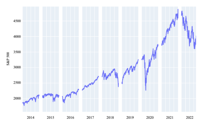
One month’s column read down is cross-sectional data: many units observed at a single point in time.
The whole grid of index values is panel/longitudinal data: every unit followed through every period. This is the most informative shape and is the combination of time series and cross-sectional data.
The most common-used file format for structured data is Comma-Separated Values (CSV). The CSV stores each item in the dataset in a single line. Variable values for each item are listed all in one line, separated by commas (“,”). The previous table in CSV format:
Region,Jan 2000,Feb 2000,Mar 2000,Pop. 2024
"New York, NY",220835,221773,222720,19940274
"Los Angeles, CA",222016,222842,223942,12927614
"Chicago, IL",156058,156202,156478,9408576
"Dallas, TX",128590,128647,128713,8344032
"Houston, TX",124446,124469,124382,7796182
2.7.2 Spatial
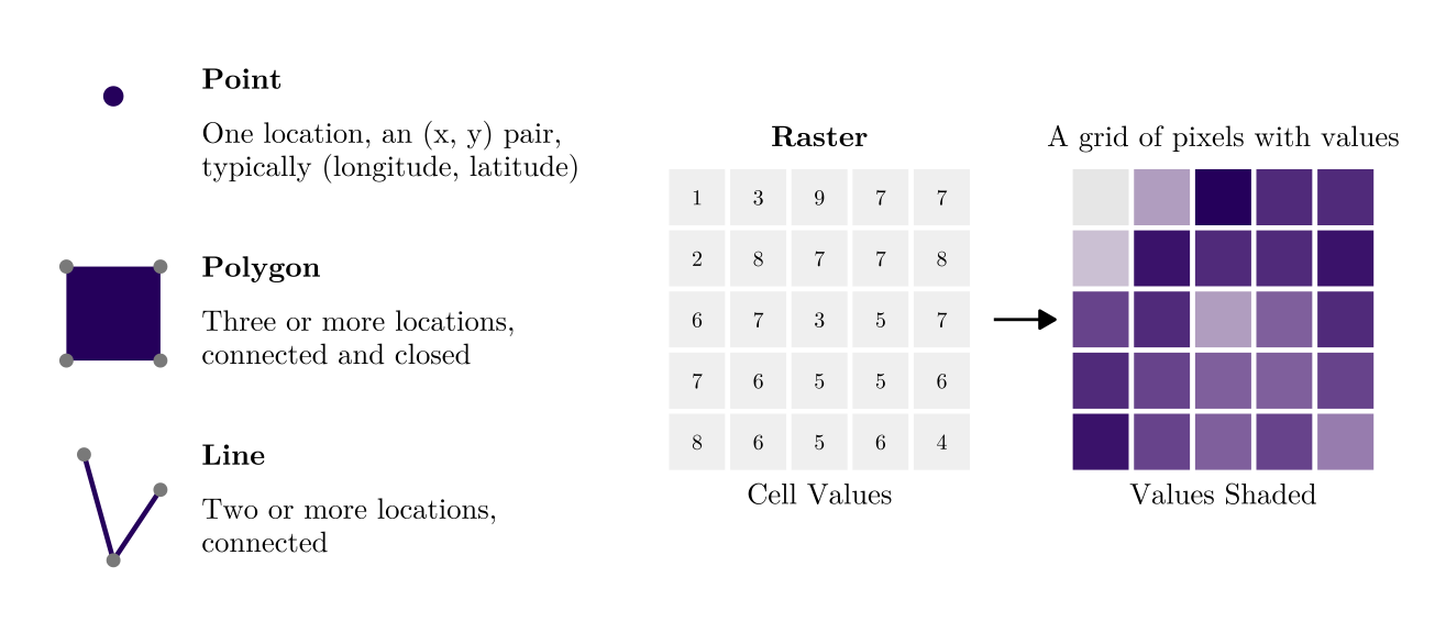
Data about physical locations and shapes of objects, including both their geographical position and attributes. Broadly speaking, there are two forms of spatial data:
Vector data is composed of discrete geometric locations, including points (a permit address), lines (a bus route), polygons (a tract boundary). The data will be in Shapefile, GeoJSON, etc.
Raster data is pixelated data where each pixel is associated with a specific geographical location. The value of a pixel can be continuous (population) or categorical (land use types). The data will be in GeoTIFF, etc.
Tobler’s First Law of Geography
Everything is related to everything else, but near things are more related than distant things.
Waldo Rudolph Tobler (1930-2018) is one of the most influential geographers and cartographers; he is also a UW alumni with undergrad, master and PhD here.
Spatial data and analysis are not the major focus of URBAN 520, we will introduce spatial statistics but for more spatial analysis and GIS software, please consider URBAN 504 and 522 instead.
2.7.3 Image/Video/Street View
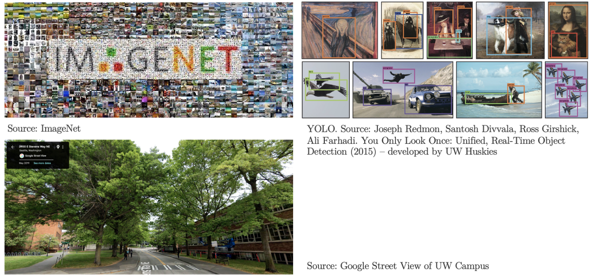
Images and videos can serve as a new data source to extract real-world information. The development of computer vision (CV) provides us new approaches, such as object detection and feature extraction, to identify the objects in images and extract features, such as the building color, building types, and quality.
2.7.4 Network
Data about the entities within a network (called nodes) and the connections or interactions between them (called edges). Network data is everywhere: social network, migration flow, infrastructure systems, etc.
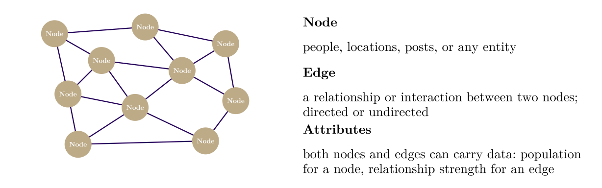
Some interesting statistics we can draw from network data, such as centrality (measure how important or influential a specific node is within the network), average path length (the average number of steps it takes to get from one node to any other node).
2.8 Who Produces Data/Numbers
In planning, data often serves as a description by design. We rely on a full count when exact figures are known (e.g., the number of parks in Seattle) and use statistical estimation when they are not (e.g., educational levels of Seattle residents). Both these estimates and any model output (like I-5 travel demand forecasts) are inherently built on assumptions.
Some numbers are gathered unintentionally. By-product data (e.g., transit tap-ins data) and administrative records (e.g., building permits applications) provide valuable insights, though they were not explicitly designed as measurements.
Most importantly, planning numbers are more than mere facts or observations. Planning balances current realities with future visions, requiring normative narratives to guide outcomes. This is why we use a standard (e.g., Seattle’s benchmark of 8 acres of parkland per 1,000 residents) and a policy target (e.g., Washington State’s goal to cut greenhouse gas emissions to 45% below 1990 levels by 2030). The following table shows some common data producers in planning.
2.9 Common Topics of Planning Data
We will work with data from various sectors because urban planning is such an interdisciplinary domain in nature. Please refer to this dataset page on the class site as a resources hub.
| Topic | Typical variables |
|---|---|
| Population | Population count Age and sex Race and ethnicity Nativity and language spoken at home Households and household type Household size Births, deaths, and net migration Migration flows between places Population projections |
| Economy and employment | Jobs by workplace location Jobs by industry Employment and wages by occupation Business establishments and payroll Household and per capita income Poverty status Labor force participation Unemployment rate Gross domestic product (GDP) Consumer prices and cost of living |
| Housing | Housing units by structure type Tenure (owner or renter) Vacancy Home values and sale prices Rents Housing cost burden Housing condition and quality Building permits and new units Subsidized housing units Mortgage applications and loans Homelessness counts and shelter beds Short-term rental listings Projected housing need |
| Land use and built environment | Parcel boundaries Land use type Zoning designation Zoning rules (lot size, height, parking, allowed housing types) Assessed land and improvement values Property sales and ownership Building footprints Building characteristics (year built, floor area, height) Density and land use mix Points of interest (shops, services, amenities, etc.) Parks and green space Land cover and impervious surface Elevation |
| Transportation | Commute mode Commute time Home-to-work commuting flows Vehicles available per household Trips by mode, purpose, and time of day Vehicle miles traveled (VMT) Road network and road condition Traffic volume (AADT) Traffic speed and congestion Transit routes, stops, and schedules Transit ridership Bicycle and pedestrian counts Walkability and transit access EV charging stations Traffic crashes, injuries, and fatalities |
| Environment | Air pollutant concentrations (PM2.5, ozone) Air quality index (AQI) Pollution sources and toxic releases Temperature and precipitation Land surface temperature and urban heat Tree canopy cover Noise exposure Greenhouse gas emissions |
| Hazards and climate | Flood zones Hazard risk scores (flood, wildfire, earthquake, heat) Expected annual losses from natural hazards Disaster declarations Storm events, deaths, and damage Flood insurance claims Precipitation frequency (design storms) Sea level rise inundation Climate projections (temperature, precipitation) |
| Health | Chronic disease prevalence (asthma, diabetes, obesity) Health behaviors (smoking, physical activity) Disability Health insurance coverage Access to health care Births Deaths and causes of death Life expectancy Food access |
| Equity and vulnerability | Social vulnerability index Area deprivation index Economic mobility (adult outcomes by childhood neighborhood) Child opportunity index Social capital and economic connectedness Displacement risk Cumulative environmental burden Local equity indices |
| Education and public services | School locations and district boundaries School enrollment School performance School staffing and finance Educational attainment College enrollment and completions Broadband availability Energy use and expenditures Energy burden Proximity to public services |
| Public safety | Reported crimes by offense type Arrests Calls for service Crime victimization Accidents and injuries |
| Finance and governance | Budgets and expenditures Capital improvement program (CIP) projects Tax revenue Property taxes Government debt Public employment and payroll Election results Voter registration and turnout |
| Emerging data | Mobile device locations and trips Visits to points of interest (foot traffic) Origin-destination flows Street-view imagery Satellite and aerial imagery Machine-learned building footprints 311 service requests Sensor readings (air quality, traffic, bicycle counters) Online listings (homes, rentals, short-term rentals) Online job postings Social media data |
2.10 Data Quality
When using some data, it would be better if:
- Use the most recently published version of the data.
- Use data sets from as unbiased a producer as possible.
- Good sources include data collected or produced by government agencies, such as the statistics compiled by the U.S. Census Bureau or the Department of Labor.
- Other top-tier data sources can include industry white papers, surveys conducted by reputable research organizations, or findings published in academic publications, such as Brookings, Urban Institute, Puget Sound Regional Council…
- Note that surveys conducted by polling agencies or think tanks, while usable, often have a political agenda, so always use discretion.
- Understand the data before everything!
- Especially for non-public access data: find out more about the data, such as how it was gathered, how old it is, and how many people were surveyed.