4 Workflows and Data Visualization
The purpose of computing is insight, not numbers.
Richard Hamming
4.1 Purposes of Data Analysis in Urban Planning
Questions that data can answer, at least in part, differ by purpose. A descriptive question asks what happened. A predictive question asks what will happen. A diagnostic question asks why it happened: an associational analysis finds associations, and a causal analysis asks whether one thing caused another. A prescriptive question asks what we should do.
4.1.1 Descriptive: What Happened?
A descriptive analysis summarizes data that already exist. It does not intend to explain why a pattern exists, or to predict.
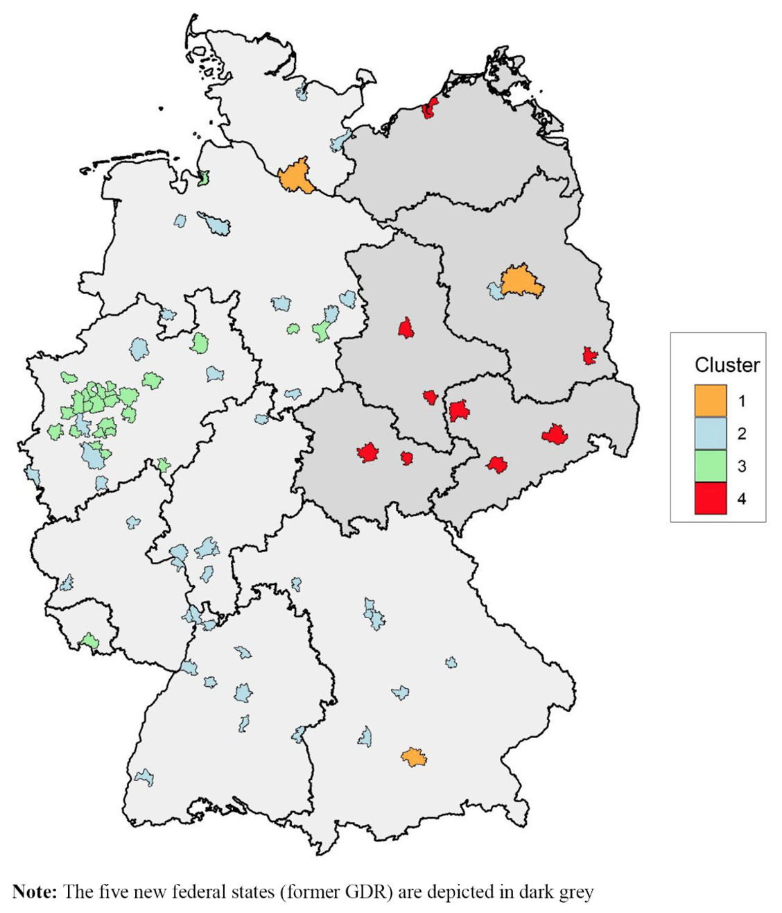
With many variables and our limited mental capacity, description itself can also based on models. For example, the study below uses two such methods to identify patterns within housing markets in German. Principal component analysis (PCA) combines correlated variables into a few components; here, 17 market variables become five. Clustering then groups places with similar values; here, German housing markets fall into four groups.
Example 4.1 Grouping German housing markets using 17 Variables \(\rightarrow\) Principal Component Analysis (PCA) \(\rightarrow\) Reduced to 5 PCs \(\rightarrow\) K-means Clustering \(\rightarrow\) Example Conclusion: German residential markets can best be segmented into four groups (Wiersma et al. 2022).
- Market size and dynamics
- Population; Population growth (%); Housing stock (no. of flats); Vacancy rate (%)
- Price level and dynamics
- Rents (EUR/sqm); Rental growth (%); Purchase prices condominiums (EUR/sqm); Purchase price growth (%); Gross initial yield (%)
- Socioeconomic indicators and dynamics
- Purchasing power per household (EUR); Purchasing power growth (%); Unemployment (%); Rent affordability (%); Price affordability; Ownership rate (%)
- Demographics
- Age cohort: 18-35 years (%); Change of age cohort: 18-35 years (%)
4.1.2 Predictive: What Will Happen?
A predictive analysis uses past data to estimate values not yet observed, such as the future sale price of a house. Prediction models, often machine learning algorithms, are judged mainly by their prediction accuracy on data they have not seen, not by whether the results can let us understand the relationship.
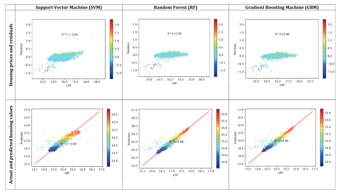
Example 4.2 The study (Ho et al. 2021) utilizes three machine learning techniques to predict the transaction price of the property in Hong Kong, using floor area, age of the property from occupation permit to sale, floor level, facing direction, and travel time to the CBD.
The models predict prices well, but they do not tell us how each variable is related to the price. Example Conclusion: Each method can achieve an accuracy at XX levels in property price prediction.
4.1.3 Diagnostic (Associational): Why Did It Happen?
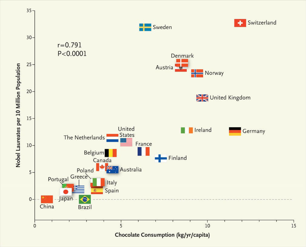
An associational analysis estimates how an outcome moves with other variables, holding the rest of the model fixed. It finds associations, so it answers “why” only in part. Across countries, for example, chocolate consumption per person is strongly correlated with the number of Nobel laureates per 10 million people (Figure 4.5). But we cannot say that in order to win more Nobel prizes, governments should start implementing chocolate promotion campaigns.
Example 4.3 This study (Thompson et al. 2023) asks how flood events and flood risk are associated with house prices, comparing two sales of the same property. Example Conclusion: the statistically significant relationship (associations) between housing prices and other variables.
| Hedonic price model coefficients | Coefficients | Significance |
|---|---|---|
| \(\beta_0\) Bracket (whether or not a pair of sales for a property occurred on either side of one or more flood events within a postcode) | 14.0% | < 0.001 |
| \(\alpha_0\) Bracket \(\times\) Risk High | -6.6% | 0.051 |
| \(\alpha_1\) Bracket \(\times\) Flood Zone | -9.4% | 0.092 |
| \(\alpha_2\) Bracket \(\times\) Flood Zone \(\times\) Risk High | -21.8% | < 0.001 |
| \(\alpha_3\) Bracket \(\times\) Flood Zone \(\times\) Flood History | 19.0% | 0.034 |
| \(\alpha_4\) Bracket \(\times\) Flood Zone \(\times\) Flood History | -12.5% | < 0.001 |
| \(\alpha_5\) Bracket \(\times\) Flood Zone \(\times\) House Type | 9.1% | 0.215 |
| \(\alpha_6\) Bracket \(\times\) Flood Zone \(\times\) Recovery | 24.2% | < 0.001 |
| \(\gamma_0\) Year of First Sale | -6.5% | < 0.001 |
| \(\gamma_1\) Year of Second Sale | 3.9% | < 0.001 |
4.1.4 Diagnostic (Causal): Why Did It Happen?
A causal analysis asks whether an intervention changed the outcome. The ideal design is a controlled experiment, like a clinical trial, in which units are randomly assigned to receive the intervention or not. In most social science and planning questions, such experiments are impossible, too costly, or unethical, so we rely on observational data and designs that approximate an experiment.
Difference-in-differences (DID) is a common one. It compares the change in a group exposed to the intervention with the change in a similar group that was not; the second group’s change stands in for what would have happened without the intervention.
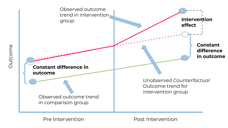
Example Conclusion: Housing purchase restriction policy in China triggered a substantial decline in the property price and transaction volume. The policy had no measurable effects on the nationwide construction boom (Cao et al. 2015).
4.1.5 Prescriptive: What Should We Do?
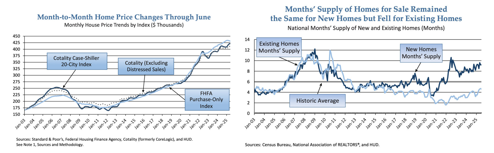
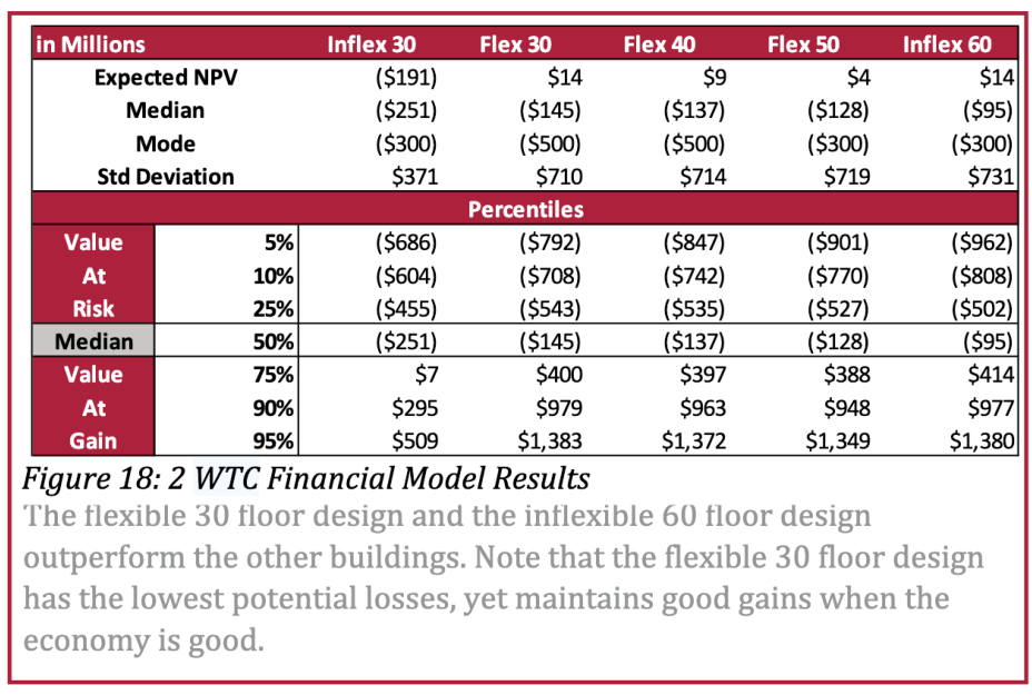
A prescriptive analysis compares possible actions and recommends one. It often simulates many future scenarios and reports the spread of outcomes for each option, so a decision can weigh expected return against risk. Leung (2014) compares five designs for one office tower by their simulated net present value (Figure 4.7). Example conclusion: under a particular condition/scenario, the expected return is XXX, while the associated uncertainty is XXX.
4.2 General Workflow of Working with Data
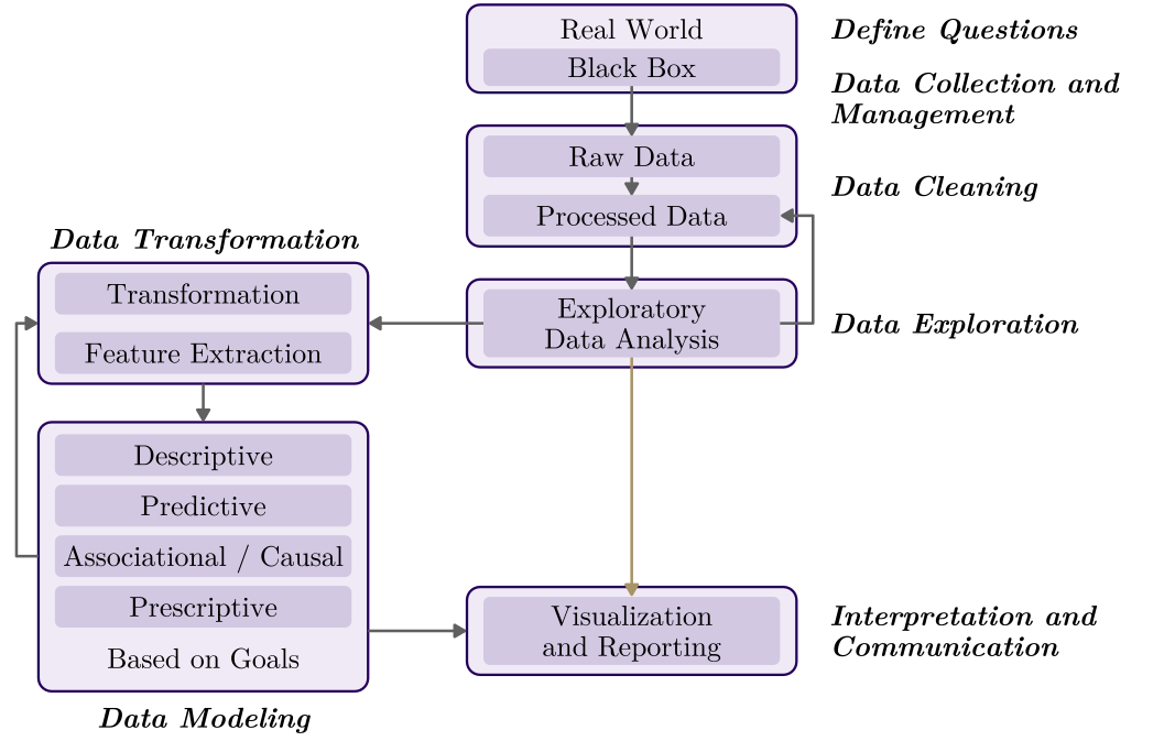
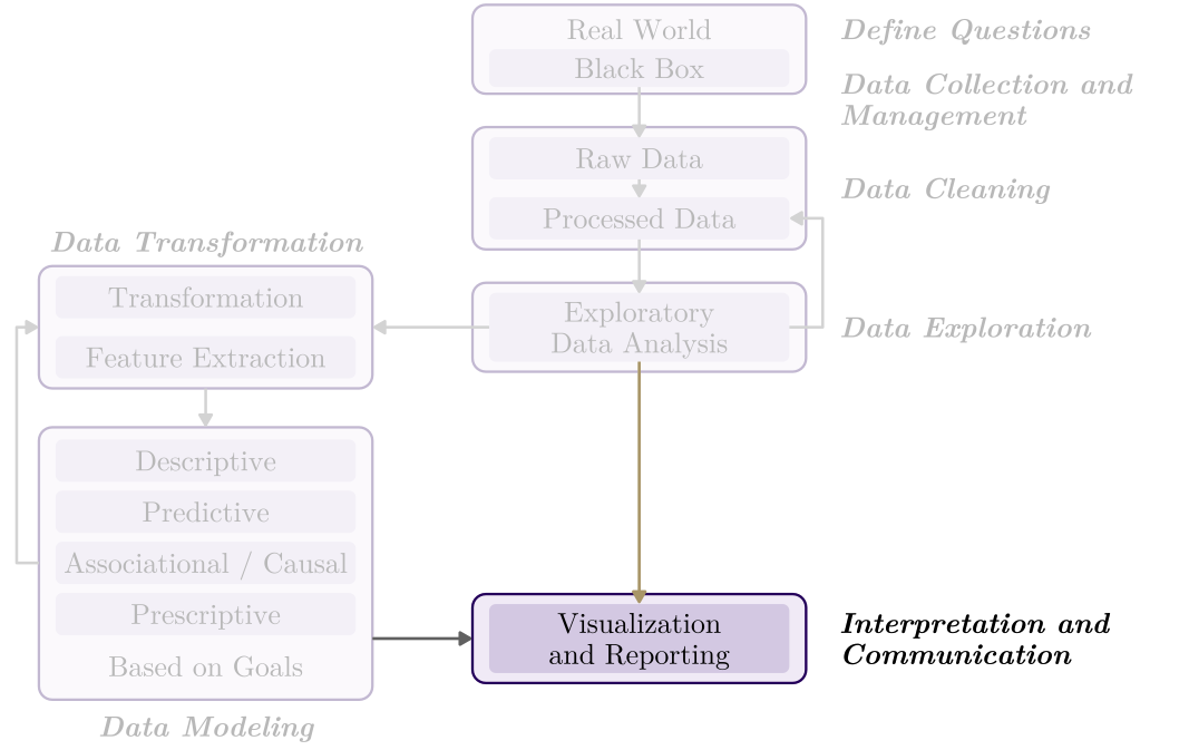
The questions can be answered through a common, but not fixed, sequence of stages, from a question about the real world to a result someone can use. The sequence is also not a straight line but an iterative process.
- Define Questions – Real World \(\rightarrow\) Black Box
- Data Collection and Management
- Data Cleaning – Raw Data \(\rightarrow\) Processed Data
- Data Exploration – Exploratory Data Analysis
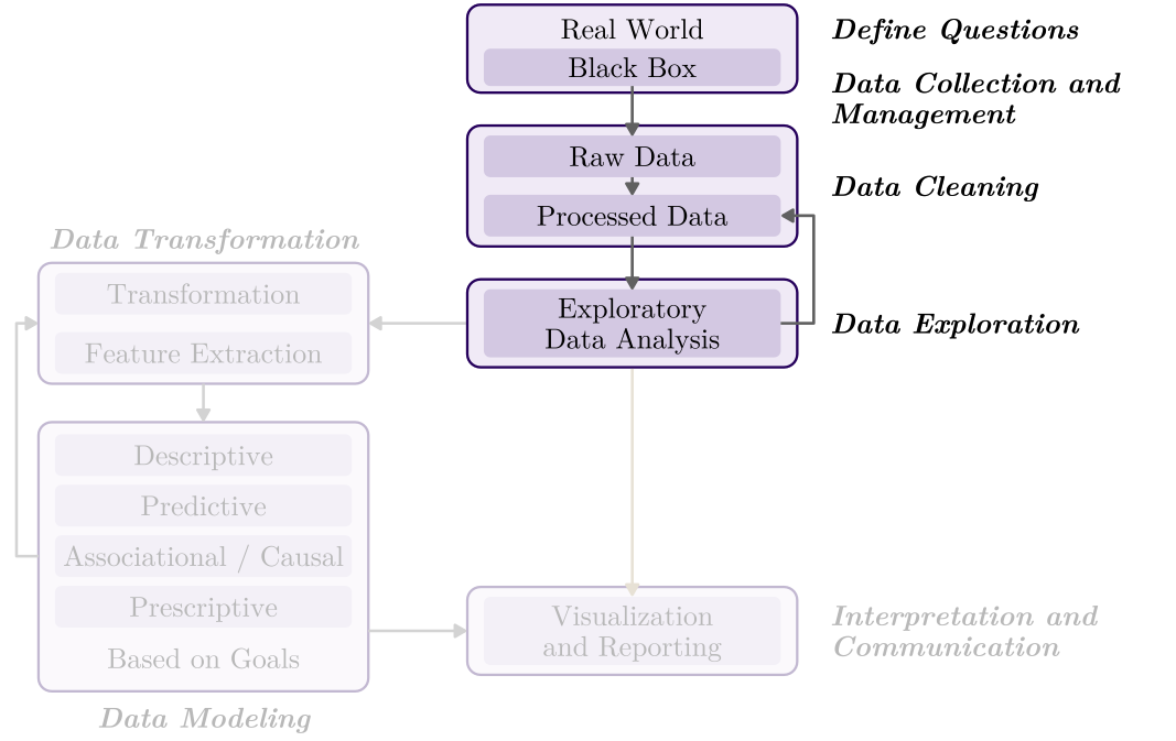
- Data Transformation – Transformation; Feature Extraction
- Data Modeling – Descriptive; Predictive; Associational / Causal; Prescriptive
- Interpretation and Communication – Visualization and Reporting
4.2.1 From Real World to Data Representation
The first four stages turn a question into a dataset we understand. The real world is a black box: we never see it directly, only through the data we choose to collect. They usually take most of a project’s time, and the choices made here shape every result that follows.
Define the questions and some key issues, such as:
- Unit of analysis (household, property, region, etc.)
- Temporal and spatial extent
- Variables, including explanatory and outcome variables
Get your data and understand it:
- The source and quality of datasets
- Population or samples? Data types? Measurements?
- Data licensing and privacy/ethics issues
- Collect data and IRB of human-subjects involved
Start to process the datasets:
- All kinds of errors in the data, such as missing values, outliers, data replication, and different spatial boundaries
- All kinds of inconsistencies in the data, such as different units, date formats, and naming styles
- Tidy data principle (we will talk about this in the lab)
Conduct exploratory data analysis:
- Explore descriptive statistics, the distribution of variables, and the relationship among variables
- Refine research questions and clean the data again if needed
4.2.2 Data Modeling
Transformation prepares the variables, and the model is then chosen by purpose.
Data transformation before modeling:
- You need to have a sense of which model to use.
- Do some numeric transformation if needed, such as log transformation, standardized
- Construct new variables if needed, such as GDP per capita
- Select the most important variables using domain knowledge, correlation, or Principal Component Analysis (PCA), etc.
Start data modeling (we classify based on purposes here):
- Descriptive (summarize what the data show)
- If the data cover the whole population, the description is the answer. If they are a sample, add inference about the population.
- Predictive (estimate values not yet observed)
- Judged by accuracy on data the model has not seen, not by whether its coefficients can be interpreted.
- Associational (how the outcome moves with other variables)
- Association, however strong or significant, is not causal relationship.
- Causal (what an intervention changes)
- Prescriptive (choose the best option)
- Usually builds on a predictive or causal model, since choosing the best option requires knowing what each option would do.
4.2.3 Visualization and Communication
An analysis is finished only when someone else can understand and use it. The last stage turns results into a message for a specific audience.
When you have some conclusions after data analysis:
- You need to explain and report your results to audiences.
- Who is your audience?
- What is the key message/takeaway?
- Make nice and effective visualizations to support your message
- Explain the results and talk about the implications
- Maybe suggest actionable steps
- Acknowledge the limitations of your analysis
4.3 Data Visualization
A good figure can show a pattern that a table hides. Visualization serves two jobs in the workflow: while exploring, it helps us find what we did not expect; when communicating, it carries a result to an audience.
4.3.1 Cholera Map
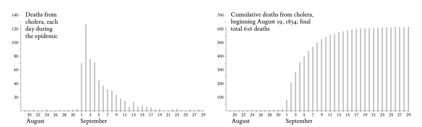
Cholera broke out in the Broad Street area of central London on the evening of August 31, 1854. John Snow, who had investigated earlier epidemics, suspected that the water from a community pumpwell at Broad and Cambridge Streets was contaminated. Testing the water from the well on the evening of September 3, Snow saw no suspicious impurities, and thus he hesitated to come to a conclusion … (Tufte 1997)
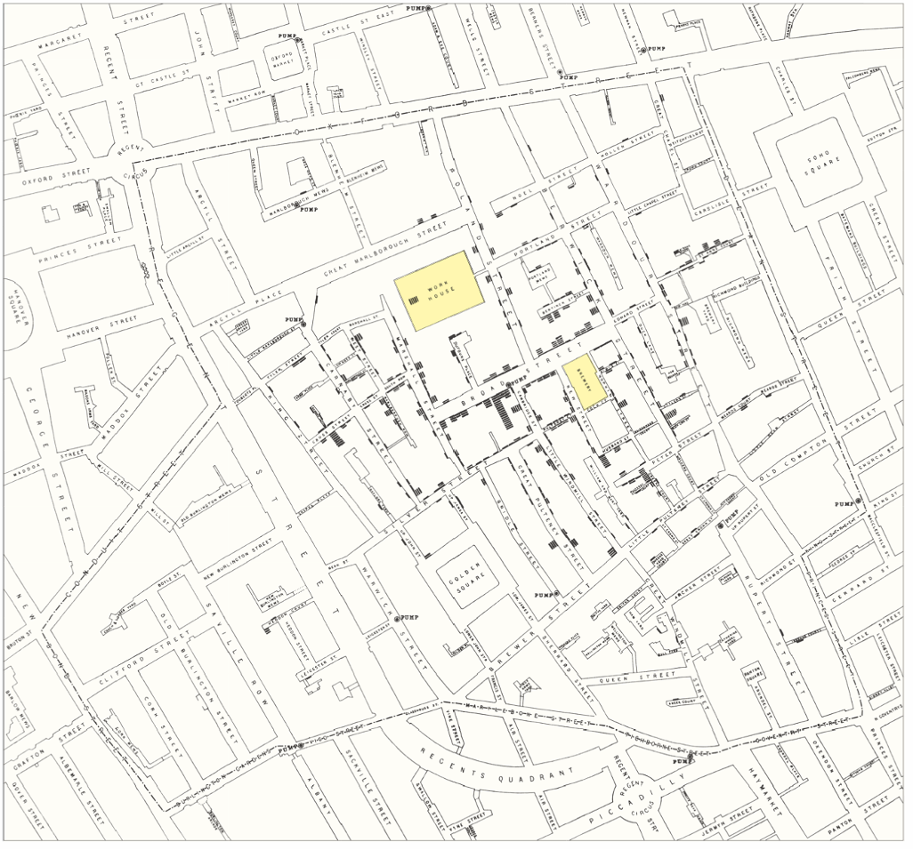
Snow then mapped the deaths, marking each one as a black bar at the victim’s address (Figure 4.13). The deaths cluster around the Broad Street pump, which pointed to the pump as the source of the outbreak.
4.3.2 Statistics Compress Information
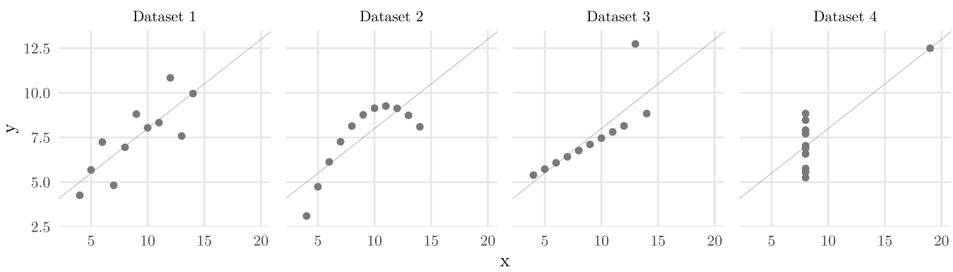
Summary statistics compress data, and the compression can hide what matters. The statistician Francis Anscombe built four small datasets that share their summary statistics: means, standard deviations, correlation, and best-fitting line. But if we plot them:
4.3.3 Explorative vs. Narrative
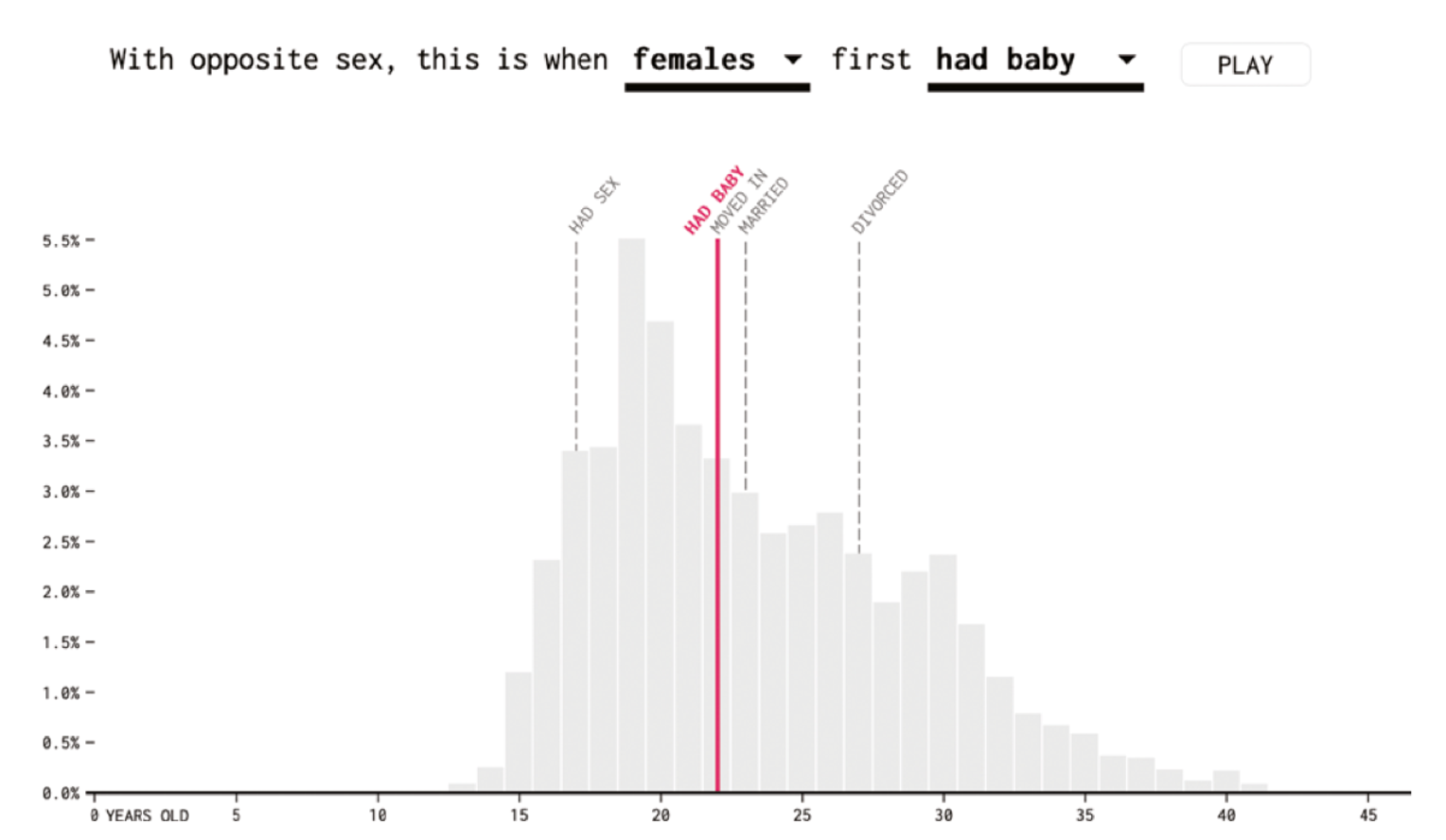
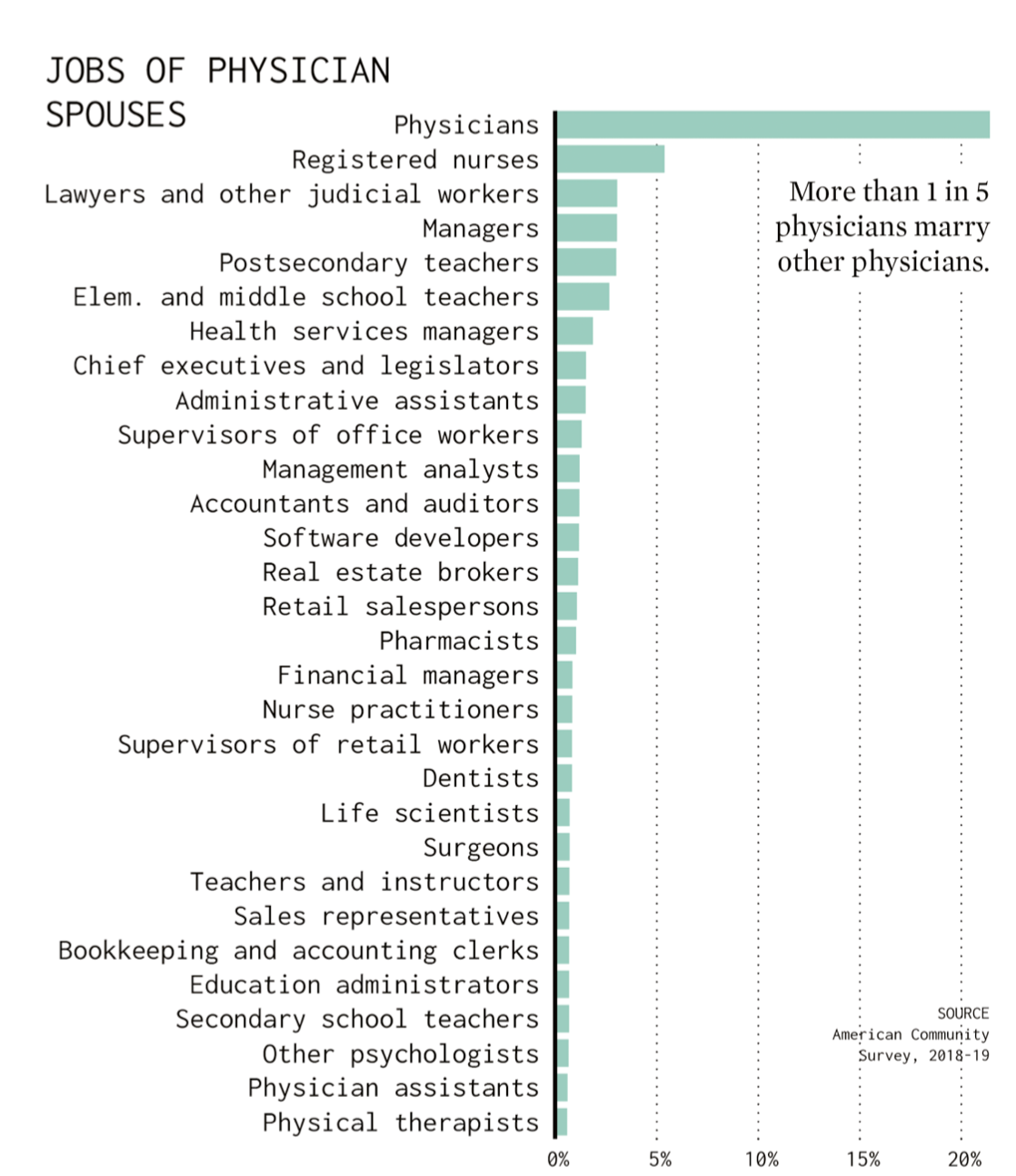
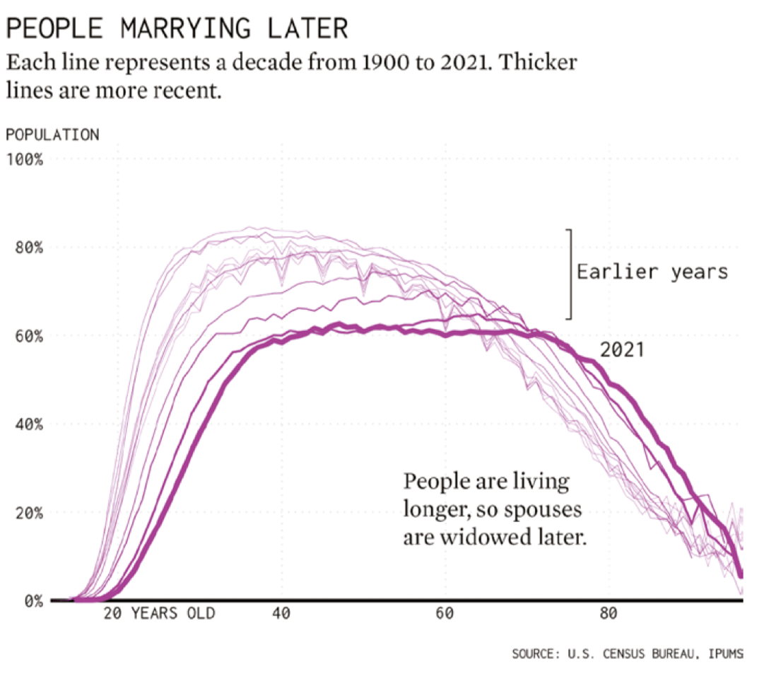
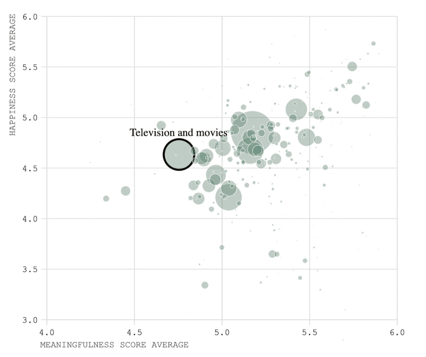
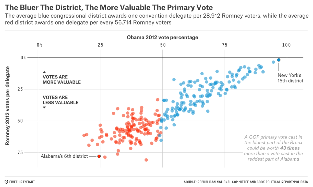
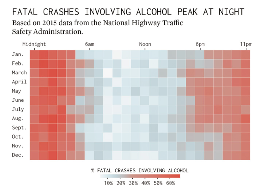
Can you tell what the differences are between these two figures?
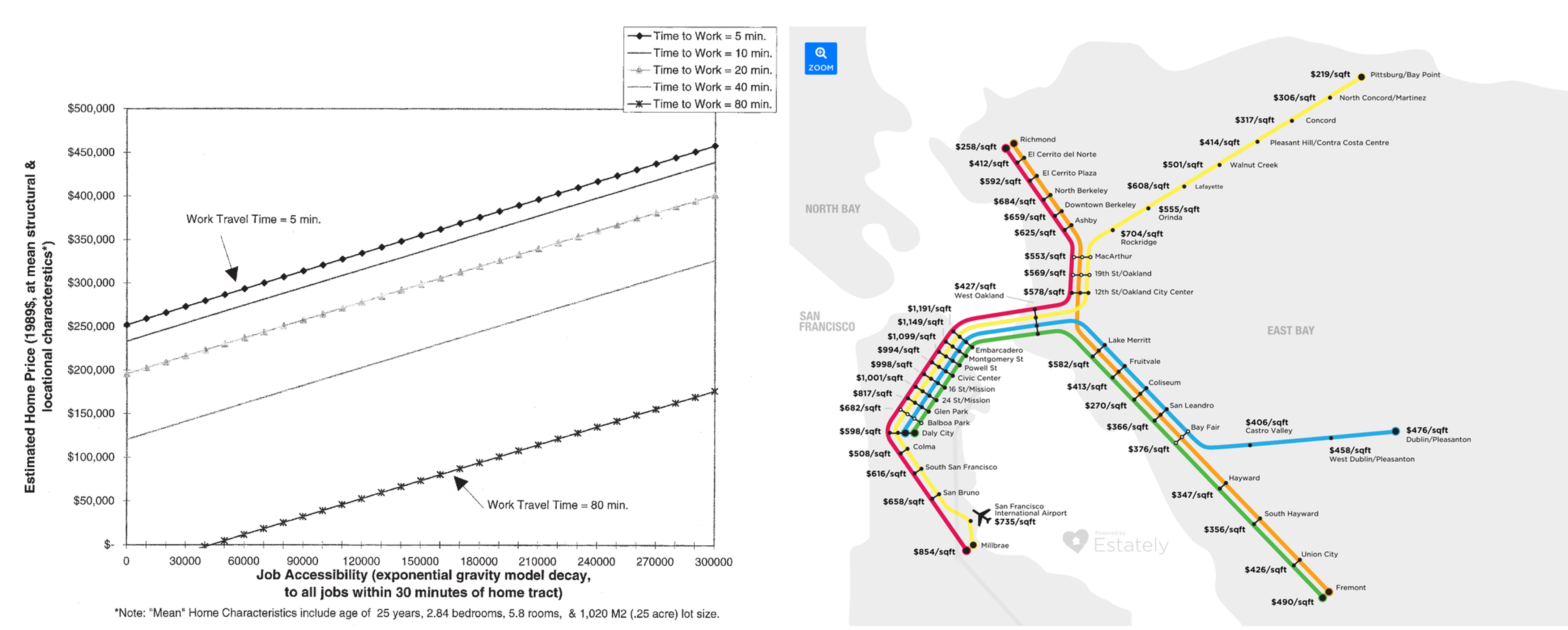
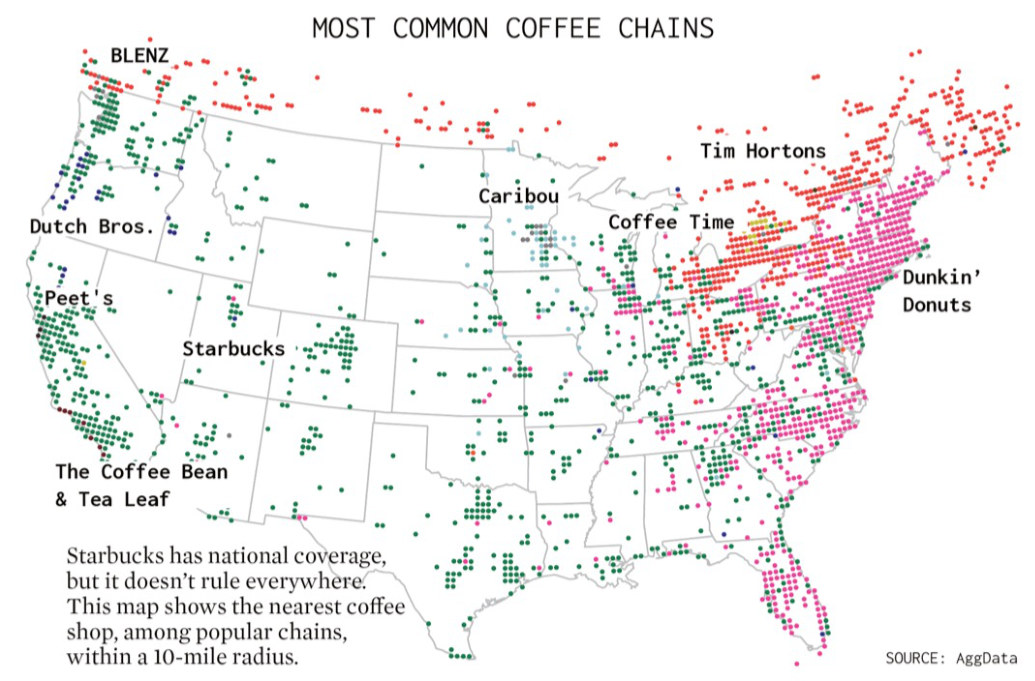
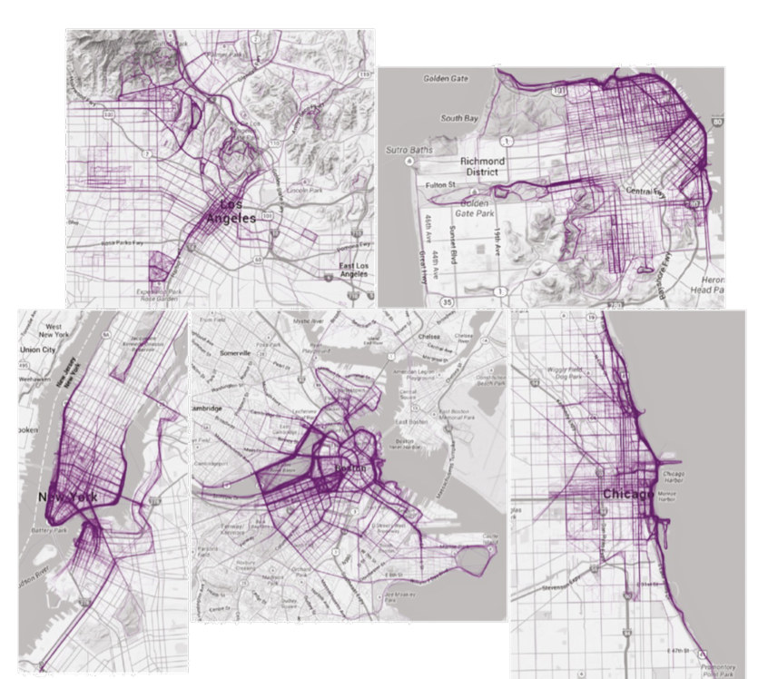
The left figure is explorative: it encodes only data and is written for researchers who will read it closely. The right figure is narrative: it borrows the BART map to catch a general reader’s eye, at the cost of precise comparison. Lankow et al. (2012) distinguish the two kinds by purpose:
| Explorative | Narrative | |
|---|---|---|
| Characteristics | Minimalist | Illustrative |
| Only includes elements that represent data | Design-focused | |
| Seeks to communicate information | Seeks to appeal to viewer with engaging visuals | |
| In the most clear, concise manner | Informs and entertains | |
| Applications | Academic research; science; business intelligence; data analysis | Publications; blogs; content marketing; sales and marketing materials |
4.4 Types of Data Visualization
4.4.1 Static
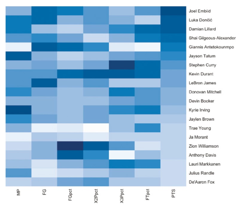
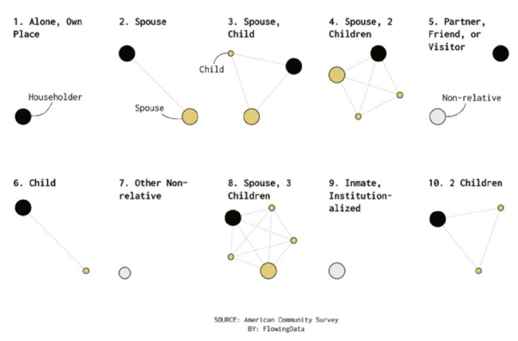
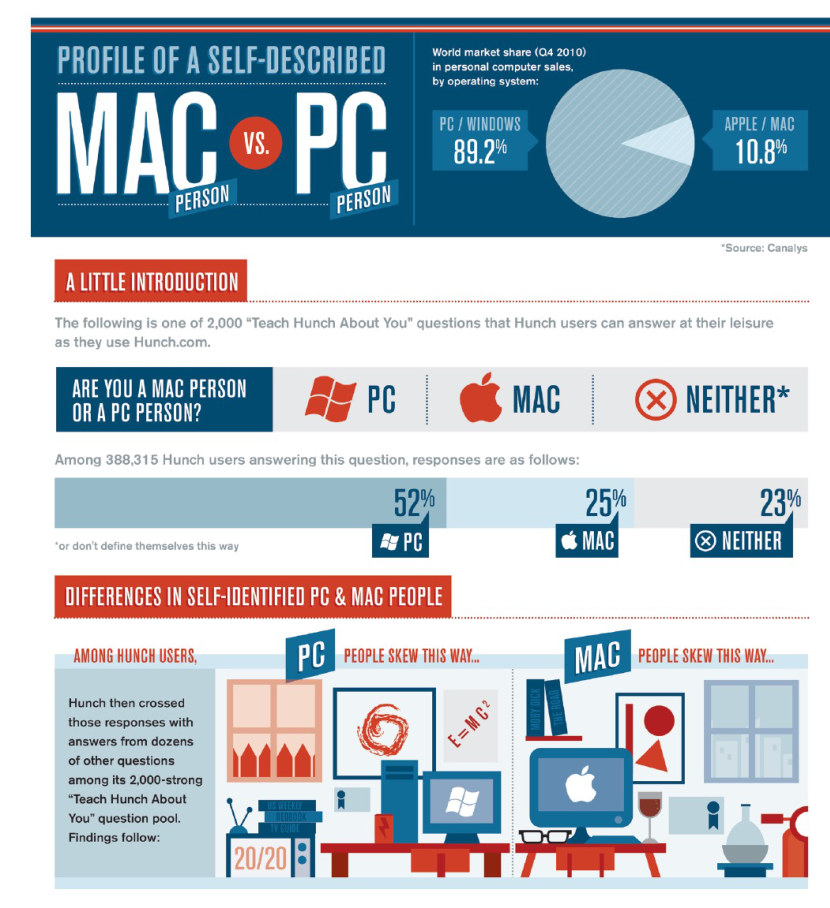
A static visualization is a still image that readers view and read (Figure 4.16). It works best as a narrative, though it can serve exploration. Most reports, plans, and slide decks use static figures, as does editorial content for blogs and social media, and they go out of date as soon as the data change.
4.4.2 Motion
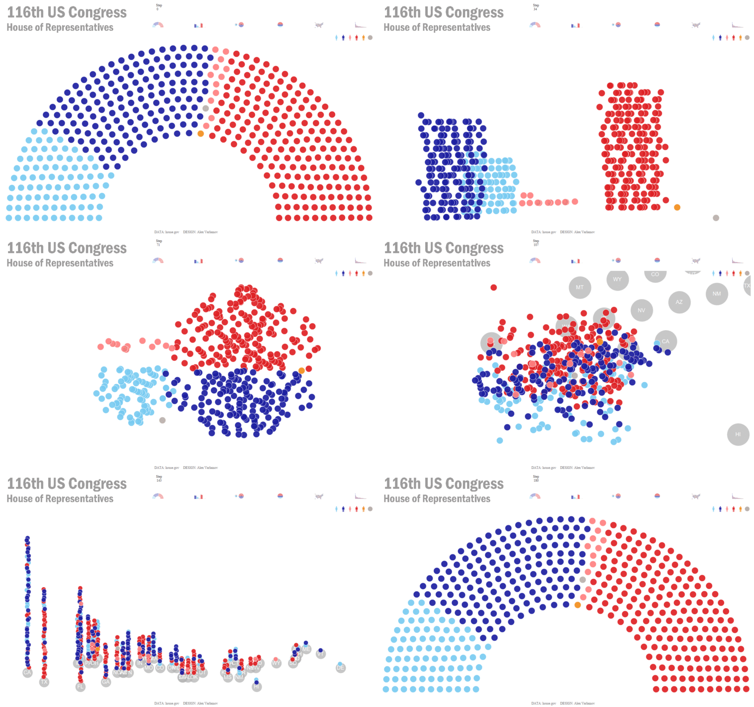
A motion visualization is animated, sometimes with a voiceover (Figure 4.17). It is almost always narrative: the viewer cannot stop to explore unless the animation is also interactive.
4.4.3 Interactive
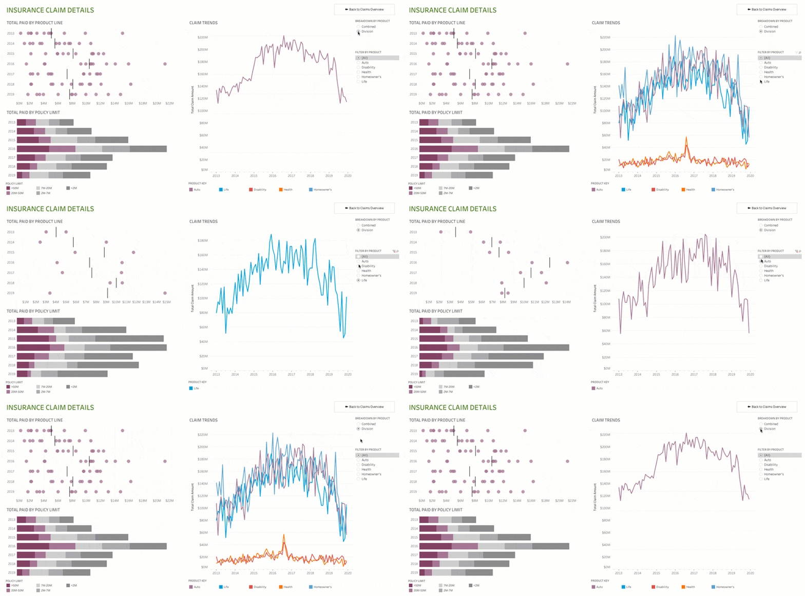
An interactive visualization lets the reader click, filter, search, and choose what to show, so it can be explorative, narrative, or both (Figure 4.18). Public agencies use dashboards and online maps for internal reports and public engagement. An interactive tool that exposes records also raises questions of data security and privacy.
4.5 More Examples of Data Visualization
We strongly recommend two online catalogues. The Data Viz Project collects chart types with examples, and lets you filter them by what a chart does. From Data to Viz starts from your data instead: choose the kind of variables you have, and a decision tree suggests charts that fit, with common pitfalls and code in R and Python.