3 Numbers in Planning
You can’t manage what you can’t measure.
Peter Drucker
Planning concepts, such as displacement risk, housing affordability, homelessness, or opportunity, are abstract and complex for ordinary people, even planners. We can qualitatively describe it for discussion or leave more room for future interpretation. But mostly, we also need quantitative indicators and indices as a shortcut to summarize. This class, we will discuss how people use indicator to define disadvantaged communities, as an example.
In California, the law requires that at least 25% of the money from the state’s Cap-and-Invest program must benefit “disadvantaged communities.”1 The state-level grant programs, such as Transformative Climate Communities, require the funded projects mainly locate in “disadvantaged communities”. Defining disadvantaged community isn’t a neutral technical activity. You can see that the action of categorization has real consequences on the communities included or excluded.
1 SB 535 (2012) created the share for disadvantaged communities. AB 1550 (2016) set the current minimums: 25% for disadvantaged communities, 5% for low-income communities or households, and another 5% for low-income communities or households within 0.5 mile of a disadvantaged community. Washington State is adopting similar programs.
3.1 From a Concept to a Framework
A concept like “Disadvantaged Community” can be interpreted simply like: a community with an annual median household income that is less than 80 percent of the statewide annual median household income.2
2 CA Water Code § 79505.5 (2025)
3 from Climate & Economic Justice Screening Tool (CEJST); has been removed by White House in early 2025.
Or complex as in CEJST 2.03: in census tracts that meet the thresholds for at least one of the tool’s categories of burden (table below), or if they are on land within the boundaries of Federally Recognized Tribes, or are surrounded by disadvantaged communities if they meet an adjusted low income threshold, or was identified as disadvantaged in the previous version, or in certain U.S. Territories that meet the low income threshold only.
| Category | Environmental, climate, or other burdens | Socioeconomic burden |
|---|---|---|
| Climate change | 1. Expected agriculture loss rate \(\geq\) 90th percentile OR 2. Expected building loss rate \(\geq\) 90th percentile OR 3. Expected population loss rate \(\geq\) 90th percentile OR 4. Projected flood risk \(\geq\) 90th percentile OR 5. Projected wildfire risk \(\geq\) 90th percentile |
Low income* |
| Energy | 1. Energy cost \(\geq\) 90th percentile OR 2. PM2.5 in the air \(\geq\) 90th percentile |
Low income* |
| Health | 1. Asthma \(\geq\) 90th percentile OR 2. Diabetes \(\geq\) 90th percentile OR 3. Heart disease \(\geq\) 90th percentile OR 4. Low life expectancy \(\geq\) 90th percentile |
Low income* |
| Housing | 1. Historic underinvestment = Yes OR 2. Housing cost \(\geq\) 90th percentile OR 3. Lack of green space \(\geq\) 90th percentile OR 4. Lack of indoor plumbing \(\geq\) 90th percentile OR 5. Lead paint \(\geq\) 90th percentile |
Low income* |
| Legacy pollution | 1. Abandoned mine land present = Yes OR 2. Formerly Used Defense Site (FUDS) present = Yes OR 3. Proximity to hazardous waste facilities \(\geq\) 90th percentile OR 4. Proximity to Superfund or National Priorities List (NPL) sites \(\geq\) 90th percentile OR 5. Proximity to Risk Management Plan (RMP) sites \(\geq\) 90th percentile |
Low income* |
| Transportation | 1. Diesel particulate matter \(\geq\) 90th percentile OR 2. Transportation barriers \(\geq\) 90th percentile OR 3. Traffic proximity and volume \(\geq\) 90th percentile |
Low income* |
| Water and wastewater | 1. Underground storage tanks and releases \(\geq\) 90th percentile OR 2. Wastewater discharge \(\geq\) 90th percentile |
Low income* |
| Workforce development | 1. Linguistic isolation \(\geq\) 90th percentile OR 2. Low median income \(\geq\) 90th percentile OR 3. Poverty \(\geq\) 90th percentile OR 4. Unemployment \(\geq\) 90th percentile |
Less than high school education > 10% |
3.1.1 CalEnviroScreen 5.0
Instead of using burden thresholds approach in CEJST, California Environmental Protection Agency (CalEPA) published the list based on a composite index, CalEnviroScreen 5.0 (CES). Its most recent 5.0 version came out on July 1, 2026. CalEPA defined disadvantaged communities as:
- Census tracts with the highest 25% of CalEnviroScreen 5.0 overall scores.
- Census tracts with the highest 5% of CalEnviroScreen 5.0 pollution burden scores.
- Census tracts that overlap at least 25% with a 2022 DAC-designated census tract based on CalEnviroScreen 4.0.4
- Lands under the control of federally recognized tribes.
4 US Census will regularly modify geographical boundaries used in census data, which leads to some confusion in data processing.
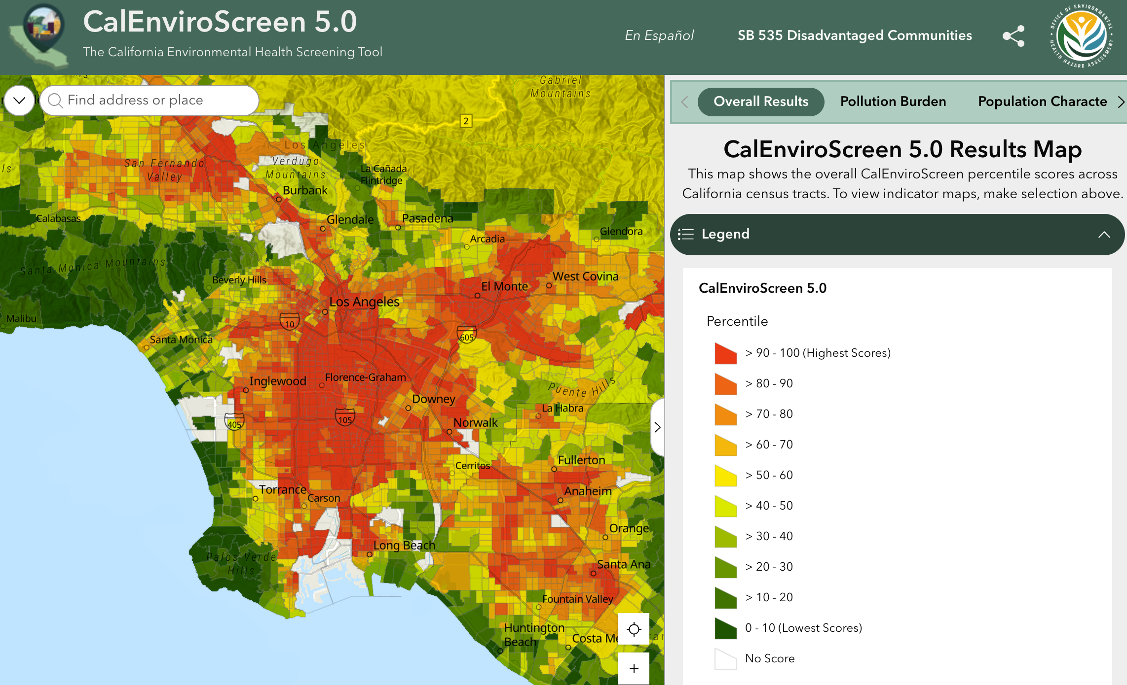
The law asked CalEPA to identify disadvantaged communities using geographic, socioeconomic, public health, and environmental hazard criteria. CalEPA and Office of Environmental Health Hazard Assessment (OEHHA) turn this into the idea of cumulative impacts: a place is more burdened with both more pollution and vulnerability.5 CES determines two major groups and four subgroups of this concept:
5 CalEPA formally defined as: Cumulative impacts means exposures, public health or environmental effects from the combined emissions and discharges, in a geographic area, including environmental pollution from all sources, whether single or multi-media, routinely, accidentally, or otherwise released. Impacts will take into account sensitive populations and socioeconomic factors, where applicable and to the extent data are available.
- Pollution Burden: exposures and environmental effects
- Population Characteristics: sensitive populations (in terms of health status) and socioeconomic conditions
The final score multiplies the two, and we will come back to it later:
\[\text{CES Final Score} = \text{Pollution Burden} \times \text{Population Characteristics}\]
3.2 Selecting Variables
CES 5.0 uses 23 indicators in those four groups and ALL of them need to be measured or counted at the census-tract level for the whole state. Some indicators can be the combination of sub-indicators. For example, Children’s Lead Risk from Housing is the combination of housing-age index and blood lead test results.6
6 Check page 58 in the CES 5.0 Technical Report for details.
You can imagine that many indicators cannot be included because they cannot be quantified (e.g., subjective well beings) or don’t cover the whole state. Some indicators are serve as proxies for the values of interest; for example, the exposure should represent what people actually breathe, drink, or touch, but no such data exist. CES can only use data on pollution sources and concentrations as indicators of potential exposure. Data availability is one of the most essential factors in composing the index, no matter how we interpreted the concept.
| Component | Group | Indicators |
|---|---|---|
| Pollution Burden | Exposures | Ozone PM2.5 Children’s lead risk from housing Diesel particulate matter Drinking water contaminants Pesticide use Toxic releases from facilities Traffic impacts |
| Environmental effects | Cleanup sites Groundwater threats Hazardous waste generators and facilities Impaired waters Small air toxic sites Solid waste sites and facilities |
|
| Population Characteristics | Sensitive populations | Asthma Cardiovascular disease Diabetes prevalence Low-birth-weight infants |
| Socioeconomic factors | Educational attainment Housing burden Linguistic isolation Poverty Unemployment |
3.2.1 How to Decide the Indicators
Before version 5.0, the OEHHA was in regular contact with academic researchers and state agencies for determining the indicators. The process has limited community engagement: gathering public inputs through workshops and written comments, once every three or four years. Starting from version 5.0, OEHHA strengthened engagement by partnering with 8 environmental community-based organizations statewide to co-design proposed updates to the tool. 7 The two new indicators, diabetes prevalence and small air toxic sites, as well as some changes, came out of a co-design process between OEHHA and community-based organizations.
7 Those organizations were selected by OEHHA based on existing relationships, prior engagement in CalEnviroScreen updates, and OEHHA knowledge of their leadership in environmental issues.
You can read the co-design process and proposed updates from this report: Mapping Local Knowledge and Experiences: Co-designing Proposed Updates to CalEnviroScreen with California Communities, January 2026 (PDF).
They established the criteria for indicator selection and also modified it:
| CES 4.0 (2021) | CES 5.0 (2026) |
|---|---|
| Indicators should provide a measure that is relevant to the component it represents, in the context of the 2005 CalEPA cumulative impacts definition. | Reflects a component of cumulative impacts with scientific rationale |
| Reflects environmental justice principles | |
| Data for each indicator should be available for the entire state at the census tract level or be translatable to the census tract level. | Data available for the entire state at the census tract level or is translatable to the census tract level |
| Indicators should represent widespread concerns related to pollution burden or population characteristics in California. | Represents a statewide, not just a regional, concern |
| Has variation across the state | |
| Informed by previous comments and feedback on CalEnviroScreen | |
| Not currently reflected in CalEnviroScreen | |
| The indicators combined together should provide a good representation of each component. | |
| Pollution burden indicators should relate to issues that may be potentially actionable by CalEPA boards and departments. | |
| Population characteristics indicators should represent demographic factors known to modify vulnerability to impacts of pollution. | |
| Data should be of sufficient quality, and be: Complete, Accurate, Current |
3.2.2 Race or Ethnicity as an Indicator?
Environmental justice research and activism always emphasize race or ethnicity as a vital factor to understand environmental burdens. However, none of the 23 indicators measures race or ethnicity. Race or ethnicity was used in CalEnviroScreen 1.0 back to 2013. And OEHHA removed race from CalEnviroScreen 1.1 to make it more widely applicable to state entities prohibited from including racial factors in their decision-making processes (Liévanos 2018).8 However, OEHHA publishes report on the analysis of the relationship between CalEnviroScreen results and race/ethnicity. You can read the CalEnviroScreen 4.0 report here.
8 California Proposition 209 prohibits state and local government entities from discriminating against or granting preferential treatment to any individual or group based on race, sex, color, ethnicity, or national origin in public employment, public education, and public contracting.
3.3 Standardization
Indicators in different units (percentages, dollars, minutes) cannot be added directly. Standardization rescales each indicator onto a common scale. Let \(y_i\) be the value of one indicator for area \(i\), with \(\bar{y}\) the mean and \(\sigma\) the standard deviation across areas. Right now we are calculating the relative position of each area instead of inferring a population parameter so those areas are the population and here is the population standard deviation.
The z-score counts standard deviations from the mean:
\[z_i \;=\; \frac{y_i - \bar{y}}{\sigma}\]
The percentile rank replaces each value by the fraction of areas at or below it; it depends only on order and is unaffected by extreme values.
Min-max rescaling stretches the range to the interval from 0 to 1:
\[r_i \;=\; \frac{y_i - \min(y)}{\max(y) - \min(y)}\]
Those are three most common-used methods and more on the page 83 of OECD et al. (2008).
3.3.1 Using Percentiles in CalEnviroScreen
Those are the rationales behind CES’s choice to use percentiles (CES 5.0 technical report):
- Ease and transparency: Percentiles are straightforward to explain and easily understandable for a wide variety of audiences.
- Varying data distributions: Indicators used in CES have varying underlying distributions, and percentile rank calculations provide a useful way to describe data without making any potentially unwarranted assumptions about those distributions.
- Consistency: Percentile scores can be applied as the normalization method to all indicators in both pollution components and population characteristic components making it a consistent approach to transform the data for every data distribution.
- Confidence in ranking of data, not in impact of magnitude: A percentile score is based on rank, not the magnitude of difference between values. … Preserving magnitude through normalization requires confidence in both raw data accuracy and the differences between values.
- Emphasis on cumulative burden: The CES score emphasizes cumulative impacts based on consistently high values across multiple indicators, not just a few extreme ones. Using a normalization method that accounts for magnitude could raise scores for tracts with fewer but extreme indicators, which would be inconsistent with the model and definition of cumulative impacts.
3.4 Building the Composite Index
After standardizing each index, we will weight the normalized values and aggregate the weighted values into one score. With \(k\) indicators, weight \(w_j\) on indicator \(j\), and \(z_{ij}\) the standardized value of indicator \(j\) in area \(i\):
\[I_i \;=\; \sum_{j=1}^{k} w_j \, z_{ij}\]
Weighting is the most subjective part of the process and has a significant effect on the overall results. One simple way is equal weighting: all variables are given the same weight. This approach implies that all variables are equally important or we don’t have enough evidence of significance of their variations.
Analytic Hierarchy Process (AHP) is another widely used method that enables the decomposition of a problem into hierarchy and assures that both qualitative and quantitative aspects of a problem are incorporated in the evaluation process, during which opinions are systematically extracted by means of pairwise comparisons.
The core of AHP is an ordinal pair-wise comparison of attributes. For a given objective, the comparisons are made per pairs of sub-indicators: Which of the two is the more important? And, by how much? The preference is expressed on a semantic scale of 1 to 9. A preference of 1 indicates equality between two sub-indicators, while a preference of 9 indicates that the sub-indicator is 9 times more important than the other one (OECD et al. 2008).
There are more methods introduced on the page 89 of OECD et al. (2008).
3.4.1 Weighting in CalEnviroScreen
In terms of CES, within each of the four subgroups, the indicator percentiles are averaged. Then, Environmental Effects counts half as much as Exposures, because it describes the presence of pollution in a community rather than exposure to it; Population Characteristics is the plain average of its two components.
\[\text{Pollution Burden} = \frac{\text{Exposures} + 0.5 \times \text{Environmental Effects}}{1.5}\]
\[\text{Population Characteristics} = \frac{\text{Sensitive Populations} + \text{Socioeconomic Factors}}{2}\]
Then, CES conducts another round of scaling/standardization: each of the two scores is divided by the highest value found in the state and multiplied by 10, so both run from 0 to 10 and count equally. The final raw score is the product (from 0 to 100) of previous two scores. After that, the tracts are ranked again.
3.4.2 Why Multiply?
Take three made-up tracts, with both components on a 0 to 10 scale.
| Tract | Pollution Burden | Population Characteristics | Added | Multiplied |
|---|---|---|---|---|
| A | 9 | 1 | 10 | 9 |
| B | 3 | 3 | 6 | 9 |
| C | 5 | 5 | 10 | 25 |
Multiplying rewards places where both kinds of burden are present at the same time. A tract with heavy pollution but few sensitive residents, or the reverse, cannot score high. This is a reflection of cumulative impact.
OEHHA’s own answer gives three reasons for multiplying (Slocombe 2026):
- Scientific Literature: Social and health conditions make pollution more harmful, so a sum understates the total. For example, the link between long-term particulate exposure and heart disease among postmenopausal women was 50 percent stronger in lower socioeconomic status neighborhoods.
- Risk Assessment Principles: Some people, such as children, can be ten times more sensitive to a chemical than others, and risk assessments already apply multipliers for that.
- Established Risk Scoring Systems: Emergency planners score risk as threat times vulnerability, and multiplying spreads the scores out more than adding does.
3.5 Sensitivity Analysis
Sensitivity analysis is the standard and also important check. Huynh et al. (2024) rebuilt CES 4.0 from its public data and changed three of those choices, one at a time and together: z-scores instead of percentiles, averaging the two components instead of multiplying them, and a few extra health indicators from CDC PLACES. On its own, each change moved 1.4 to 5.4% of all tracts across the DAC line. Across all the combinations, 16.1% of tracts were a DAC under some models but not under others, while only 25% are designated at all. At the 75th percentile cutoff, a tract’s rank could vary by 44 percentile points across models, and even tracts near the 5th percentile could qualify under a slightly different model. Please refer to the section on “UNCERTAINTY AND SENSITIVITY ANALYSIS” within OECD et al. (2008).
3.6 Determine the Threshold
The 2026 disadvantage community list has four parts (OEHHA):
- Census tracts with the highest 25% of CalEnviroScreen 5.0 overall scores.
- Census tracts with the highest 5% of CalEnviroScreen 5.0 pollution burden scores.
- Census tracts that overlap at least 25% with a 2022 DAC-designated census tract based on CalEnviroScreen 4.0.
- Lands under the control of federally recognized tribes.
Under the first rule, the tract ranked 2,259th is in, the tract ranked 2,260th is out, and the two are almost the same. Huynh et al. (2024) estimates the effects of such designation: roughly doubled a tract’s funding (+104%, 95% CI 62 to 145%), about $2.08 billion over four years for 2,007 tracts (designated as DAC).
Recall that the law require 25% money from Cap-and-Invest should go to disadvantaged communities. However, when we calculate the number of tracts and population within and without designated disadvantaged communities (DACs):
So the 2026 list covers about 29% of Californians. If programs only met the 25% floor and spread the money per person, a DAC resident would get about ~20% less than a resident elsewhere, the opposite of what the targeting is meant to do.
3.7 U.S. Census Data
Four of the five socioeconomic indicators come straight from the ACS, and OEHHA pulled them through the Census Bureau’s API in R.
| Indicator | Table | Years |
|---|---|---|
| Educational attainment | ACS B15003 | 2020–2024 |
| Linguistic isolation | ACS C16002 | 2020–2024 |
| Poverty | ACS C17002 | 2020–2024 |
| Unemployment | ACS B23025 | 2020–2024 |
3.7.1 U.S. Constitution
The United States Constitution mandates in Article I, Sections 2 and 9, that a complete enumeration of the US population be taken every 10 years.
The actual enumeration shall be made within three years after the first meeting of the Congress of the United States, and within every subsequent term of ten years, in such manner as they shall by law direct.
AKA the decennial census (https://www.census.gov/programs-surveys/decennial-census.html) and it only asks few questions of everyone. However, 10 years is a long time to wait for new information…
3.7.2 American Community Survey (ACS)
The American Community Survey (ACS) is a survey of 3.5 million US households annually (~3% of the US population). Far more detailed than the decennial census and more timely.
Through the ACS, we know more about jobs and occupations, educational attainment, veterans, whether people own or rent their homes, and other topics. Public officials, planners, and entrepreneurs use this information to assess the past and plan the future. When you respond to the ACS, you are doing your part to help your community plan for hospitals and schools, support school lunch programs, improve emergency services, build bridges, and inform businesses looking to add jobs and expand to new markets, and more.
Census Reporter https://censusreporter.org is an open and free website to make U.S. Census Bureau data easier to explore and use.
| Collection period | Geographies covered | Years of data in the 2024 estimates |
|---|---|---|
| 1 year | Population > 65,000 | 2024 |
| 5 years | All major geographies down to block group | 2020-2024 |
- These are estimates, so note the margin of error!
- Be cautious when working with very small subgroups (ex., American Indian or Alaska Native) or geographies with low populations. The estimates may lose much of their meaning.
| Geography | Geographic Area Name | Estimate!!Total: | Margin of Error!!Total: |
|---|---|---|---|
| 1400000US06001400100 | Census Tract 4001, Alameda County, California | 3035 | 402 |
| 1400000US06001400200 | Census Tract 4002, Alameda County, California | 1983 | 209 |
Geography is GEOID. Margin of Error!!Total is 90% confidence interval and we will cover this in later chapters and it is a measure of uncertainty.
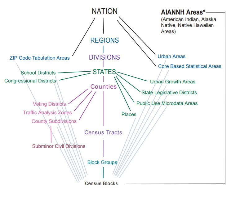
3.7.3 Levels of Geographic Aggregation
Nested hierarchy of geographic boundaries (each level tiles exactly into the one above):
- Nation
- State
- County
- Census tract
- Census block group
- Census block
Sometimes, we may also use school districts, municipal boundaries, zip code areas, or statistical areas. They do not nest in this hierarchy. Be careful when you combine data with different geographic boundaries.
3.7.4 GEOID
Every census geography carries a GEOID that encodes its ancestry. For example, 53-033-005303-2-034 is a block in UW campus:
GEOIDs and their boundaries shift between censuses, so be careful and any multi-year comparison must state which GEOID it uses.
3.7.5 A Note on Race/Ethnicity in the Census
The census codes race (White, Black or African American, American Indian or Alaska Native, Asian, Native Hawaiian or Other Pacific Islander) separately from Hispanic or Latino origin, which is an ethnicity: a person of any race can be Hispanic.