6 Exploratory Data Analysis
Exploratory data analysis is detective work.
John W. Tukey, Exploratory Data Analysis (1977)
Exploratory data analysis (EDA) is the first look at a dataset that attempts to identify general patterns in the data. We may or may not have a fixed research question at this stage. The purpose of EDA is understanding the data, including its sources, producer, potential quality issues, patterns, relationships among variables. EDA will guide us toward the next stage of data modeling or visualization.
This lecture, including the lab sessions, will explore the sales of single-family houses and townhomes in King County, Washington, from 1999 through 2025. Andy Krause built the file from the public records of the King County Department of Assessments and distributes it as the data package kingCoData. Today, we will discuss EDA along with this dataset as the example.
6.1 Data Overview
Before computing anything, we should understand where the data come from, what one row/column stands for, and overall descriptive statistics of the data.
6.1.1 Where the Data Come From
Every transfer of real estate in Washington is reported on a real estate excise tax affidavit (REET Affidavit), the form filed with the county when the real estate excise tax is paid. The King County Department of Assessments compiles the county’s affidavits into a sales file and publishes it, together with its parcel, building, and tax-roll files, on its data download page. Andy Krause’s processing scripts join these files and keep only sales between unrelated parties on the open market, of single-family houses and townhomes1.
1 Krause kept only sales that look like ordinary market transactions of a single-family house or townhome. He achieved this by removing condominiums and multi-unit buildings; transfers that are not market sales, such as those between relatives, by gift, or through foreclosure, bankruptcy, or a tax sale; sales of several parcels at once; and sales of $50,000 or less.
6.1.2 What One Row Stands For
The unit of observation is what one row describes. It is a sale (or transaction) in this data: the 605,614 rows describe 347,905 properties, of which 180,024 appear once and 167,881 appear two or more times. The unit a research question needs, the unit of analysis, can differ from the unit of observation. We could reach it by manipulating data (e.g., aggregating rows), for example to one row per property or one row per year.
Two columns identify rows. sale_id is an unique ID or primary key, which can be used to identify sales. pinx identifies the property and we can use it to links each sale to the property’s record, which makes it a foreign key.
| Column | Row 1 | Row 2 | Row 3 |
|---|---|---|---|
sale_id |
1999..144 | 1999..258 | 1999..379 |
pinx |
..2734100475 | ..1535200725 | ..9214400005 |
sale_date |
1999-01-05 | 1999-01-05 | 1999-01-08 |
sale_price |
$150,000 | $235,000 | $190,000 |
sale_nbr |
1 | 1 | 1 |
sale_warning |
(blank) | (blank) | (blank) |
join_status |
demo | demo | demo |
join_year |
1999 | 1999 | 1999 |
latitude |
47.5444 | 47.4212 | 47.6829 |
longitude |
-122.3208 | -122.4381 | -122.2989 |
city |
SEATTLE | KING COUNTY | SEATTLE |
present_use |
2 | 2 | 2 |
land_val |
$21,000 | $46,000 | $79,000 |
imp_val |
$66,000 | $132,000 | $139,000 |
year_built |
1900 | 1916 | 1947 |
year_reno |
0 | 0 | 0 |
sqft_lot |
4000 | 6695 | 5184 |
sqft |
1410 | 990 | 1570 |
sqft_1 |
760 | 990 | 900 |
sqft_fbsmt |
0 | 0 | 200 |
grade |
7 | 6 | 7 |
fbsmt_grade |
0 | 0 | 6 |
beds |
3 | 2 | 4 |
bath_full |
1 | 1 | 2 |
wfnt |
0 | 0 | 0 |
6.1.3 What Each Column Measures
The original data has 48 columns and in this lecture, we keep 25 of them to make it simpler. Table 6.2 is the data dictionary of the 25 columns.
| Column | Meaning | Format | Level of measurement |
|---|---|---|---|
sale_id |
Identifier of the sale: the year, two dots, and a number | text | nominal |
pinx |
Parcel number of the property, with two dots in front | text | nominal |
sale_date |
Date on the sale document | date | interval |
sale_price |
Price paid, in dollars of the year of the sale | integer | ratio |
sale_nbr |
Which recorded transfer of the property this sale was, counting from 1999 (1 = the first); NA if the property has only one recorded transfer. The count includes transfers the publisher removed from the file | integer | ordinal |
sale_warning |
Assessor warning codes, separated by spaces; codebook | text | nominal |
join_status |
What happened to the house between 1999 and 2025, relative to the sale (Table 6.9) | text | nominal |
join_year |
Year of the assessor record the building columns come from (including all variables below), 1999 or 2025 | interval | nominal |
latitude |
Location of the parcel: latitude | decimal | interval |
longitude |
Location of the parcel: longitude | decimal | interval |
city |
City, or KING COUNTY for unincorporated area | text | nominal |
present_use |
Use of the parcel; codebook | integer | nominal |
land_val |
Assessed value of the land, in dollars of the record year | integer | ratio |
imp_val |
Assessed value of the building, the “improvement”, in dollars of the record year | integer | ratio |
year_built |
Year the house was built | integer | interval |
year_reno |
Year of the last major renovation; 0 if none | integer | interval |
sqft |
Total living area, in square feet | integer | ratio |
sqft_1 |
Living area of the first floor, in square feet | integer | ratio |
sqft_fbsmt |
Finished basement area, in square feet; 0 if none | integer | ratio |
fbsmt_grade |
Quality of finished basement, on the scale of grade; 0 if none |
integer | ordinal |
grade |
Building quality; codebook | integer | ordinal |
beds |
Number of bedrooms | integer | count |
bath_full |
Number of full bathrooms | integer | count |
wfnt |
Body of water a waterfront lot faces, 0 if none; codebook | integer | nominal |
sqft_lot |
Lot area, in square feet | integer | ratio |
6.1.4 A First Look at the Values
| Column | Min | Median | Mean | Max | Zeros | Missing |
|---|---|---|---|---|---|---|
sale_price |
$50,293 | $475,000 | $628,827 | $63,000,000 | 0.0% | 0 |
land_val |
$0 | $397,000 | $500,171 | $35,124,000 | 0.7% | 0 |
imp_val |
$0 | $421,000 | $531,479 | $33,860,000 | 0.7% | 0 |
sqft |
0 | 1,980 | 2,136 | 22,370 | 0.0% | 0 |
sqft_1 |
20 | 1,200 | 1,258 | 11,790 | 0.0% | 0 |
sqft_fbsmt |
0 | 0 | 296 | 11,560 | 60.3% | 0 |
sqft_lot |
0 | 7,466 | 13,994 | 9,539,640 | 0.0% | 0 |
beds |
0 | 3 | 3.4 | 54 | 0.0% | 0 |
bath_full |
0 | 2 | 1.6 | 21 | 1.0% | 0 |
sale_nbr |
1 | 2 | 2.2 | 22 | 0.0% | 125,018 |
year_built |
1900 | 1978 | 1974 | 2025 | 0.0% | 0 |
year_reno |
0 | 0 | 63 | 2025 | 96.9% | 0 |
latitude |
47.155 | 47.565 | 47.550 | 47.778 | 0.0% | 0 |
longitude |
-122.528 | -122.222 | -122.211 | -121.157 | 0.0% | 0 |
| Column | Stored as | Distinct values | Min | Mode | Max | Zeros | Missing |
|---|---|---|---|---|---|---|---|
sale_id |
text | 605,614 | — | — | — | — | 0 |
pinx |
text | 347,905 | — | ..1336801005 | — | — | 0 |
sale_date |
date | 9,635 | 1999-01-01 | 2004-05-24 | 2025-12-31 | — | 0 |
sale_warning |
text | 202 | — | (blank) | — | — | 0 |
join_status |
text | 8 | — | nochg | — | — | 0 |
join_year |
decimal | 2 | 1999 | 2025 | 2025 | 0.0% | 0 |
city |
text | 41 | — | SEATTLE | — | — | 0 |
present_use |
integer | 3 | 2 | 2 | 29 | 0.0% | 0 |
grade |
integer | 14 | 1 | 7 | 20 | 0.0% | 0 |
fbsmt_grade |
integer | 14 | 0 | 0 | 13 | 60.3% | 0 |
wfnt |
integer | 9 | 0 | 0 | 9 | 98.6% | 0 |
6.2 Data Cleaning and Processing
6.2.1 Missing Values
Missing values do not always look missing. We can find several forms of missing in this data:
- Explicit missing values,
NA, such assale_nbrfor 125,018 sales (20.6%). - Blank text:
sale_warningis blank for 90.1% of sales. - Zero for “none” or “does not apply”:
year_renois 0 for 96.9% of sales (never renovated),sqft_fbsmtis 0 for 60.3% (no finished basement), andwfntis 0 for 98.6% (not on the water). - Zero for unknown: for example, both
land_valandimp_valare 0 for 3,965 sales, with a median sale price of $368,000.
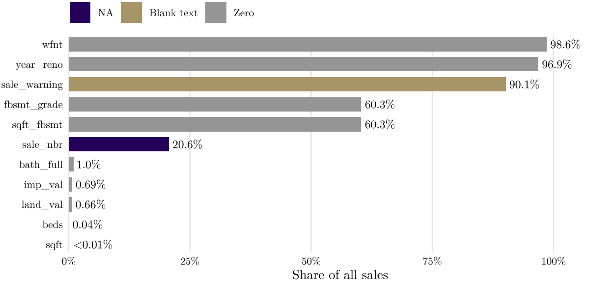
What to do with these missing values? There is no single answer but probably, we can consider doing: recode sale_nbr from NA to 1; turn year_reno into a yes-or-no variable, renovated or not; set land_val and imp_val to missing where both are 0.
6.2.2 Dealing with Missing Data
Three mechanisms are usually distinguished the reason of data missing (OECD et al. 2008):
Missing completely at random (MCAR): whether a value is missing has nothing to do with any variable, observed or not. For example, the missing values in variable income would be of the MCAR type if (i) people who do not report their income have, on average, the same income as people who do report income; and if (ii) each of the other variables in the data set would have to be the same, on average, for the people who did not report their income and the people who did report their income.
Missing at random (MAR): missingness depends on variables we do observe, but not the variable of interest. For example, the missing values in income would be MAR if the probability of missing data on income depends on marital status but, within each category of marital status, the probability of missing income is unrelated to the value of income.
Missing not at random (MNAR): missingness depends on the missing value itself. For example, high income households are less likely to report their income.
OECD et al. (2008) briefly organizes the ways of dealing with missing values into three groups:
Case deletion, also called complete-case analysis: drop every case with a missing value in the variables used. The result is unbiased only under MCAR, and the sample shrinks. As a rule of thumb, the handbook advises against deleting cases when a variable has more than 5% of its values missing.
Single imputation: replace each missing value with one value, such as the mean, median, or mode of the column, the median of a group of similar cases, a value copied from a similar case, or a value predicted from other variables.
Multiple imputation: fill each missing value several times, so that the uncertainty about the filled-in values carries into the results.
It goes beyond this course but it’s an important problem for data science. If you are interested in missing data, you can refer to this book: Statistical Analysis with Missing Data.
6.2.3 Impossible and Suspicious Values
Some values are almost impossible for some variables, age of 200 is a quite suspicious data record. We can set up a few rules for different datasets, for example, in our data:
- Range: a value lies in a plausible interval, such as 0 to 15 bedrooms, or a price above zero.
- Cross-field: the values in one row agree with each other, such as a first floor no larger than the whole living area.
- Temporal: dates come in a possible order, such as a house built before it is sold.
- Referential: a code exists in its lookup table, such as a warning code that appears in the assessor’s list of codes.
- Format and pattern: values should meet particular format, such as a standard US zip code must be exactly 5 digits long.
| Rule | Kind | Sales that fail |
|---|---|---|
| Bedrooms at most 15 | Range | 5 |
| Living area above 0 | Range | 2 |
| First floor no larger than the living area | Cross-field | 438 |
| Built no later than the year of the sale | Temporal | 13,261 |
| Every warning code listed in the assessor’s code table | Referential | 18 |
6.2.4 Duplicates
It is possible to have duplicate data records, we can identify some patterns:
- Exact duplicates: data records are identical in every column.
- Key duplicates: data records share same unique ID or primary key.
- Near duplicates: one case entered twice with small differences, such as two spellings of one address or two unique ID for one transaction.
- Legitimate duplicates: duplicate on purpose so need to make decisions.
The sales file has no exact duplicates but there are 2,427 properties that has two or three sales on the same day, 4,859 rows in all. The following table shows one such case.
sale_id |
pinx |
sale_date |
sale_price |
sale_nbr |
sale_warning |
|---|---|---|---|---|---|
| 2000..42139 | ..0011200350 | 2000-11-25 | $303,000 | 2 | 40 |
| 2000..42140 | ..0011200350 | 2000-11-25 | $303,000 | 1 | 41 |
Possible explanation is when an employer moves an employee to another city, a relocation company often buys the employee’s house and resells it to the final buyer. The two sales are recorded on the same day with the same price. Whether such cases should be treated as duplicate depends on the research questions and domain knowledge.
6.2.5 Outliers
An outlier is a value far from most of the others. It may be an error ($4,500 entered for $450,000), a different kind of case (a whole apartment building sold as one parcel), or a real extreme. Two common approaches in statistics to find outlier are:
- IQR approach (see box-plot section below): beyond \(Q_1 - 1.5 \times \text{IQR}\) and \(Q_3 + 1.5 \times \text{IQR}\)
- z-score: beyond \(\bar{y} - 3 \times s\) and \(\bar{y} + 3 \times s\), where \(\bar{y}\) is the sample mean and \(s\) the sample standard deviation; in z-scores, \(|z_i| > 3\) with \(z_i = (y_i - \bar{y}) / s\)
For this data, we can believe that most rows identified by the two approaches above are not errors, even though the rules flag them: they are real sales of expensive homes, and a long tail of high prices is the nature of the housing market. Meanwhile, domain knowledge tells us that a property with 54 bedrooms is likely a data mistake. Domain knowledge guides these decisions: the rules only flag values that lie far from the rest, and knowledge of the subject tells us whether a flagged value is an error, a different kind of case, or a real extreme.
| Rule | Scale | Low cutoff | High cutoff | Sales below | Sales above |
|---|---|---|---|---|---|
| IQR fences | dollars | below $0 | $2,677,500 | 0 | 989 |
| IQR fences | log dollars | $235,303 | $4,557,945 | 7 | 177 |
| z-score beyond 3 | dollars | below $0 | $4,527,628 | 0 | 180 |
| z-score beyond 3 | log dollars | $210,378 | $5,428,517 | 5 | 108 |
6.2.6 Recoding and Derived Variables
Recoding maps codes to labels or merges categories. A derived variable is computed from other columns. The following table shows some variables:
| New variable | Made from |
|---|---|
| Type | present_use: 2 and 6 single-family, 29 townhome |
| Sale year, sale month | sale_date |
| Price per square foot | sale_price divided by sqft |
| Age at sale | sale year minus year_built |
| Renovated | year_reno greater than 0 |
| Place | city, with KING COUNTY read as unincorporated |
| Price in 2025 dollars | sale_price and a price index |
A ratio inherits the problems of its denominator. Price per square foot is unstable for very small houses. Also we may consider doing log transformation to variables (such as the sale prices) which are right-skewed in order to make the distribution more symmetric.
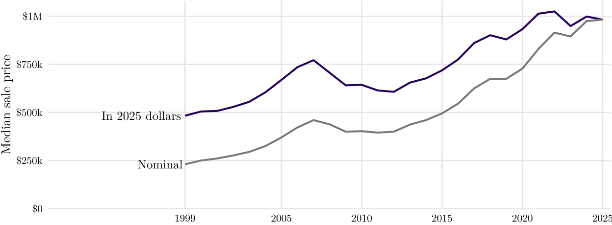
Here, we adjusted all prices for inflation. A dollar in 1999 bought more than a dollar in 2025 so the common practice is to convert the dollars in records to the dollars of one reference year using a price index (such as Consumer Price Index for All Urban Consumers, CPI-U, for Seattle-Tacoma-Bellevue, the data from Bureau of Labor Statistics). We will talk more about money in future sessions.
6.2.7 Joining, Aggregating, and Reshaping
Joining combines multiple tables through keys, as Andy joined the sales to the parcel, building, and tax records. Each sale was matched to the assessor’s records of its parcel from 1999 or from 2025, labeled with what happened to the house between the two (join_status), and given the building columns of the record judged closer to the house that was sold.
join_status |
What happened to the house | Record from | Sales |
|---|---|---|---|
nochg |
Existed in 1999, no major change since | 2025 | 377,507 |
new |
New house on a parcel created after 1999 | 2025 | 160,060 |
miss99 |
Existed in 1999, missing from the 1999 records | 2025 | 7,581 |
reno - before |
Renovated before the sale | 1999 or 2025 | 18,505 |
reno - after |
Renovated after the sale | 1999 | 8,605 |
demo |
Demolished after the sale | 1999 | 11,077 |
rebuilt - after |
Rebuilt after the sale (may be a land sale) | 2025 | 9,632 |
rebuilt - before |
Rebuilt before the sale | 1999 | 12,647 |
Aggregating collapses rows into aggregated units, such as one row per property, per year, or per city, and so changes the unit of analysis.
Reshaping changes the layout of the same values, such as reshaping a data to meet the principle of tidy data: each row is one observation and each column one variable (Wickham, Tidy Data, 2014). We will discuss more in the lab.
6.3 Univariate Analysis
The next step in Exploratory Data Analysis (EDA) is to examine how the values of different variables are distributed. Graphical approaches for examining the distribution of the data include histograms, boxplots, cumulative distribution functions, and quantile-quantile (Q-Q) plots. Information on the distribution of values is often useful for selecting appropriate analyses and confirming whether assumptions underlying particular methods are supported (e.g., normally distributed residuals for a least squares regression).
6.3.1 Histograms
A histogram summarizes the distribution of the data by placing observations into intervals (also called classes or bins) and counting the number of observations in each interval. The y-axis can be number of observations, percent of total, fraction of total (or probability), or density (in which the height of the bar multiplied by the width of the interval corresponds to the relative frequency of the interval).
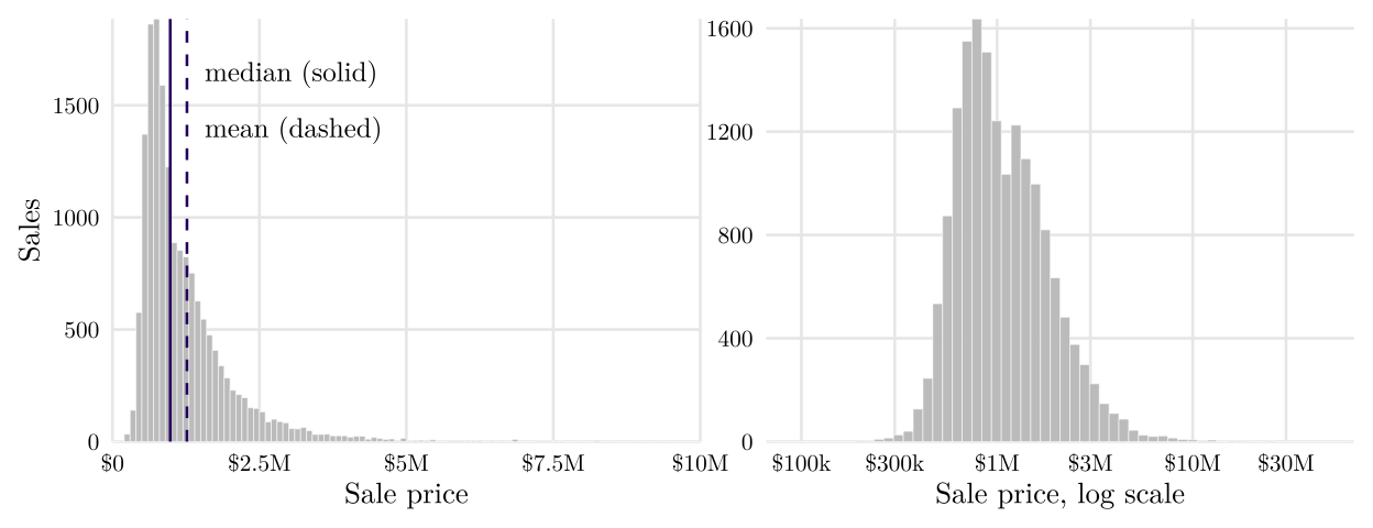
On a linear dollar axis, the 2025 price distribution is heavily right-skewed. When plotted on a log scale, the same prices normalize into a single, distinct peak centered near $1 million. The visualization utilizes a log axis labeled with original dollar values, capturing the principle that equal geometric distances represent equal percentage changes rather than absolute differences.
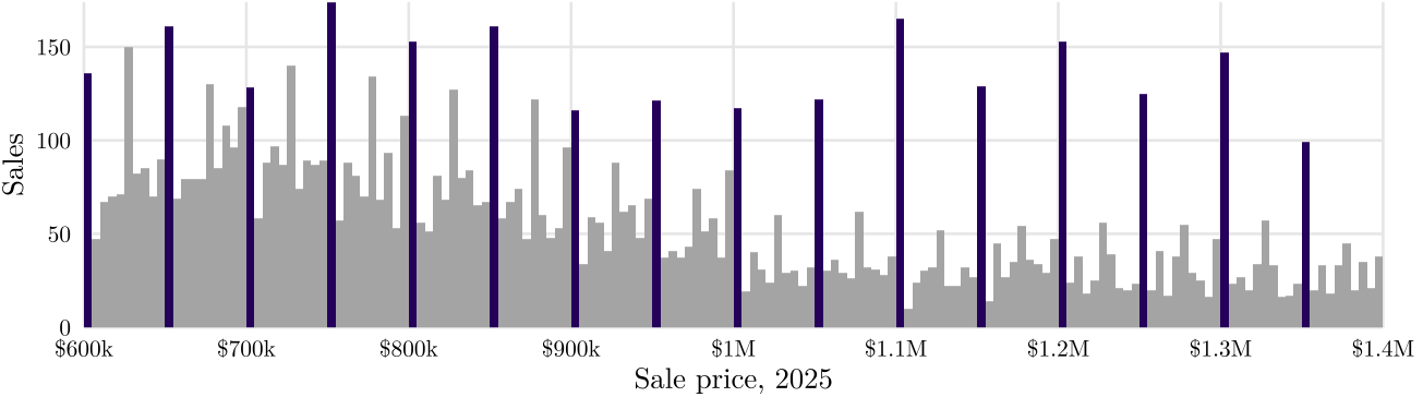
The width of the bins is also a choice, and one dataset drawn at different widths can look like different distributions. Bins that are too wide merge real groups; bins that are too narrow show noise.
Narrow bins also show heaping, values piling up on round numbers. In 2025, 25.3% of the prices are multiples of $50,000, and the $5,000 bins that start at such a multiple hold 137.9 sales on average, against 53.2 for the others.
6.3.2 Box Plots
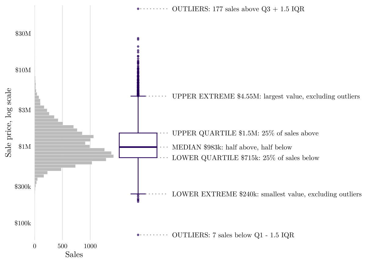
A box and whisker plot (also referred to as boxplot) provides a compact summary of the distribution of a variable. A standard boxplot consists of:
- a box defined by the 25th and 75th percentiles
- a horizontal line or point on the box at the median
- vertical lines (whiskers) drawn from each hinge (quartile) to the extreme value.
- \(Q_1 - 1.5 \times IQR\) and \(Q_3 + 1.5 \times IQR\)
- the interquartile range (IQR) is calculated as 75th percentile - 25th percentile
- outliers: any observation outside this whiskers
6.3.3 Cumulative Distribution Functions
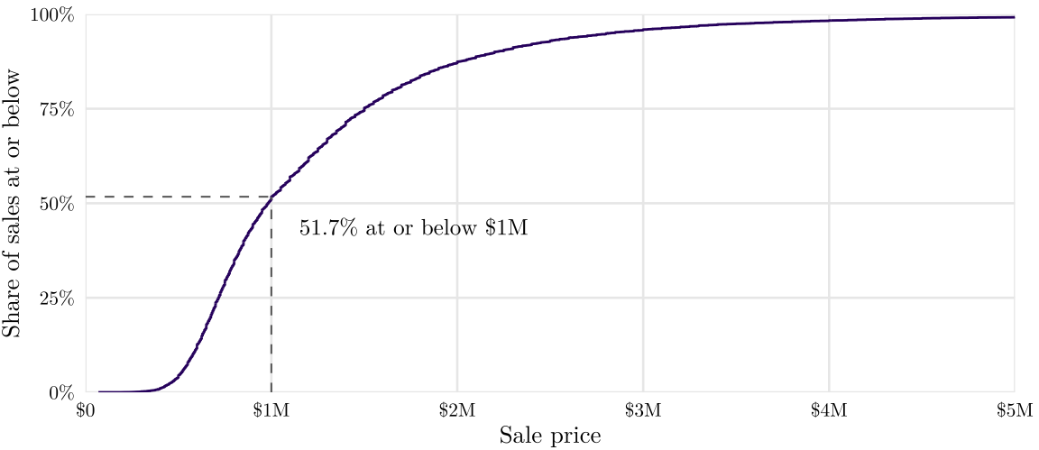
The cumulative distribution function (CDF) gives, for every value \(x\), the share of the cases at or below it:
\[F(x) = \frac{\text{number of cases with a value at or below } x}{n}\]
Drawn from data, the empirical CDF is a monotonically increasing function ranging from 0 to 1. Fundamentally, a CDF fully characterizes and uniquely determines a probability distribution. Furthermore, when the distribution is continuous, the derivative of the CDF is the probability density function (PDF), which represents the continuous, idealized counterpart to the frequency histogram. We will talk about this in future sessions.
6.3.4 Q-Q Plots
A quantile-quantile (Q-Q) plot compares the shape of a distribution with a reference shape, usually the normal distribution. It plots the sorted values against the values the reference would put at the same positions. Points on a straight line mean the same shape; points curving up at the right end mean a long right tail; an S shape means heavy tails on both sides; flat steps mean repeated values.
6.3.5 Bar Charts
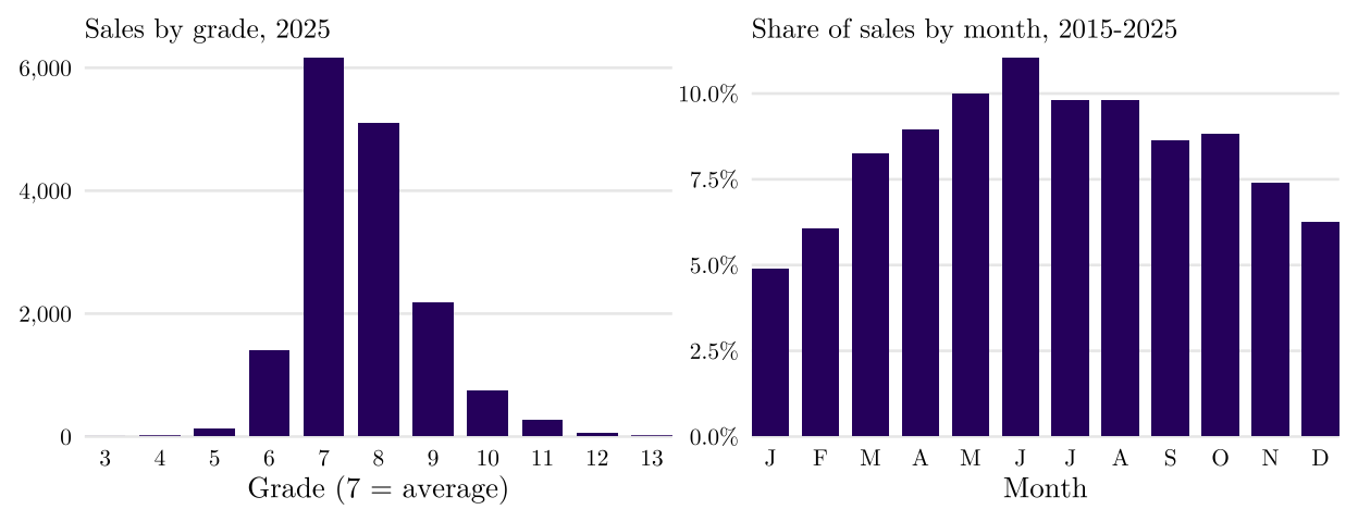
A categorical variable is summarized by a frequency table and drawn as a bar chart. Sort nominal categories by their counts, keep ordinal categories in their order, merge rare categories into “other”, and give the counts behind any shares.
6.4 Multivariate Analysis
This section looks at two variables at a time, then at several at once, and then at what a third variable can do to a comparison of two.
6.4.1 Scatterplots
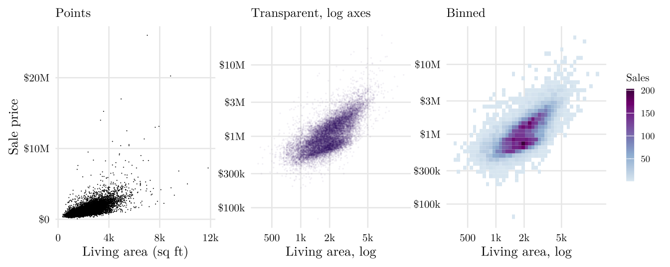
A scatterplot draws one point per case, with one numerical variable on each axis. With thousands of points, overplotting hides the densest parts of the cloud; smaller points, transparency, log axes, jitter for values that come in steps, and binning the plane into cells all help.
6.4.2 Scatterplot Matrix
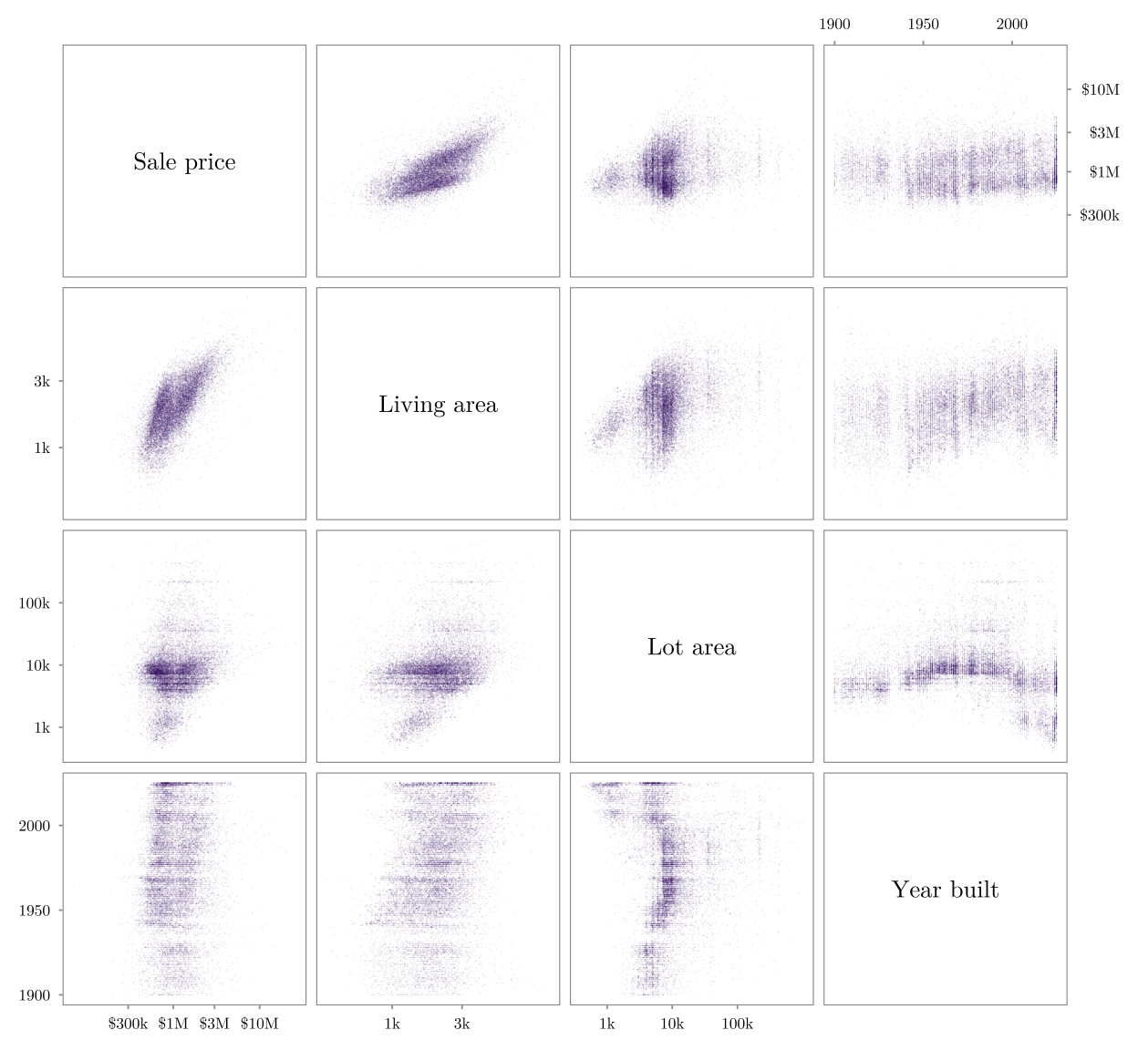
A scatterplot matrix draws every pair of several numerical variables at once:
6.4.3 A Numerical and a Categorical Variable
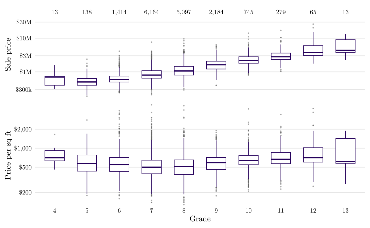
Compare the distribution of the numerical variable across the categories with side-by-side box plots, one histogram per group, or a strip plot of all the points, and keep the group sizes in view.
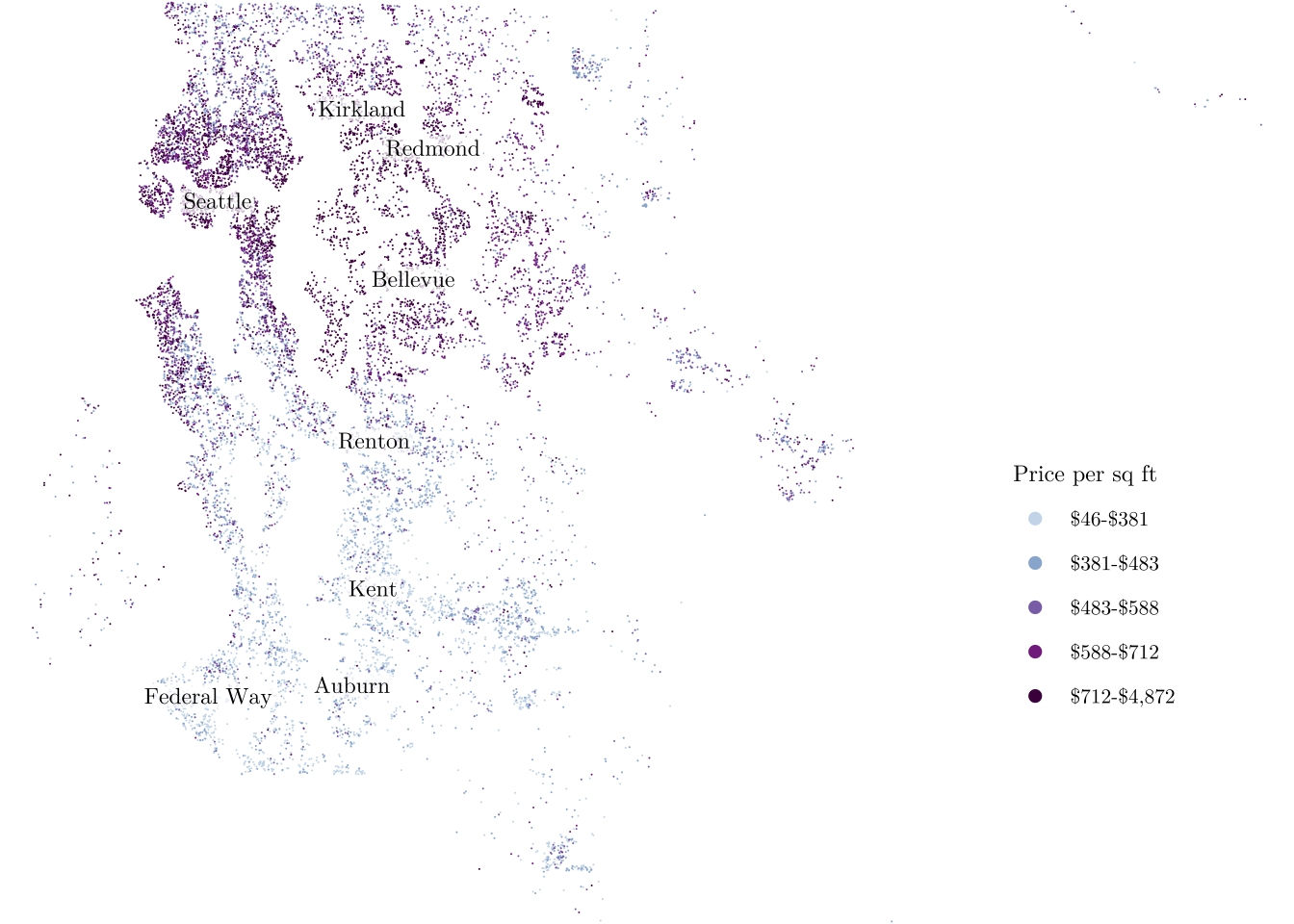
A map is the same comparison with location as the grouping.
6.4.4 Two Categorical Variables
A contingency table counts the cases in each combination of two categorical variables.
| Single-family | Townhome | Total | |
|---|---|---|---|
| Seattle | 3,826 | 1,207 | 5,033 |
| Rest of King County | 10,671 | 409 | 11,080 |
| Total | 14,497 | 1,616 | 16,113 |
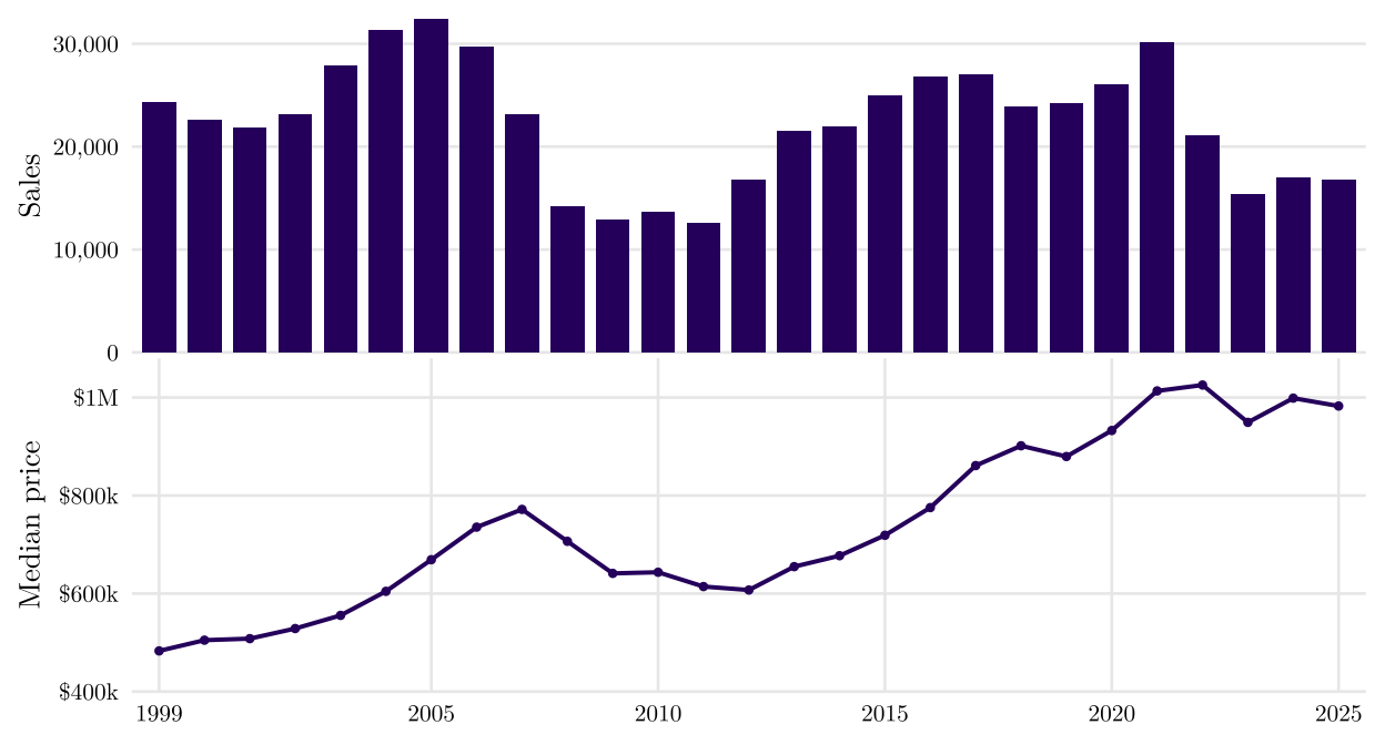
6.4.5 Time as a Variable
Time is drawn in order, as a line or as bars. Ask what is counted at each time, a level such as the median price or a flow such as the number of sales, and remember that a yearly summary also reflects which homes sold that year.
6.4.6 A Third Variable
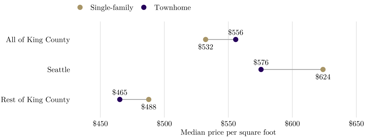
Stratification repeats a comparison inside groups defined by a third variable. It can reverse a comparison, which is called Simpson’s paradox. Across the county, townhomes sold for more per square foot than single-family houses ($556 against $532), yet inside Seattle ($576 against $624) and in the rest of the county ($465 against $488) they sold for less.
The reason is where they sell: 74.7% of the townhome sales are in Seattle, where every kind of house costs more per square foot. Reading a relationship among individuals off data about areas is a related trap, the ecological fallacy.