7 Basic Probability
Probability theory is nothing but common sense reduced to calculation.
Pierre-Simon Laplace
7.1 Logic Reasoning
We have believed in Geocentrism for centuries until Nicolaus Copernicus proved earth is not the center of the universe. To shift from the old geocentric view to the new heliocentric model, scientists relied heavily on different ways of thinking.

7.1.1 Deduction
Deduction and induction are two different approaches to reasoning and drawing conclusions. Deduction starts with a general principle or theory and applies it to specific cases to derive conclusions. If the general principle is true, then the conclusion must also be true. For example: \[ \text{All men are mammal} + \text{Mark is a man} \longrightarrow \text{Mark is a mammal} \]
7.1.2 Induction
Induction begins with specific observations or data and uses them to formulate general principles or theories. This conclusion is not guaranteed to be true, but because of the observations, we more likely believe that conclusion is true. For example: \[ \begin{aligned} &\text{The first 5 eggs are rotten} + \text{all eggs have the same production date} \\&\qquad \overset{?}{\longrightarrow} \text{the next egg is rotten} \end{aligned} \]
7.1.3 Deduction and Induction
Deduction is more creditable than induction, as it is based on logical reasoning and established principles. But we are still using induction all the time, as we cannot always have a general principle or theory to apply. We saw the sun rise in the east every day, and we concluded that the sun always rises in the east. But these conclusions are not guaranteed to be true, as we did not observe it all days.
Our conclusions always implicitly base on an assumption that all unobserved cases will behave like the observed cases. David Hume, a Scottish philosopher, pointed out that this assumption is not logically justified. You can see that this assumption also comes from induction and we cannot prove it in anyway. So, we can have an argument that: even through it is not logically justified, but the chance of this assumption being true is very high. That is also right for sun rising in the east tomorrow. But what if this case:
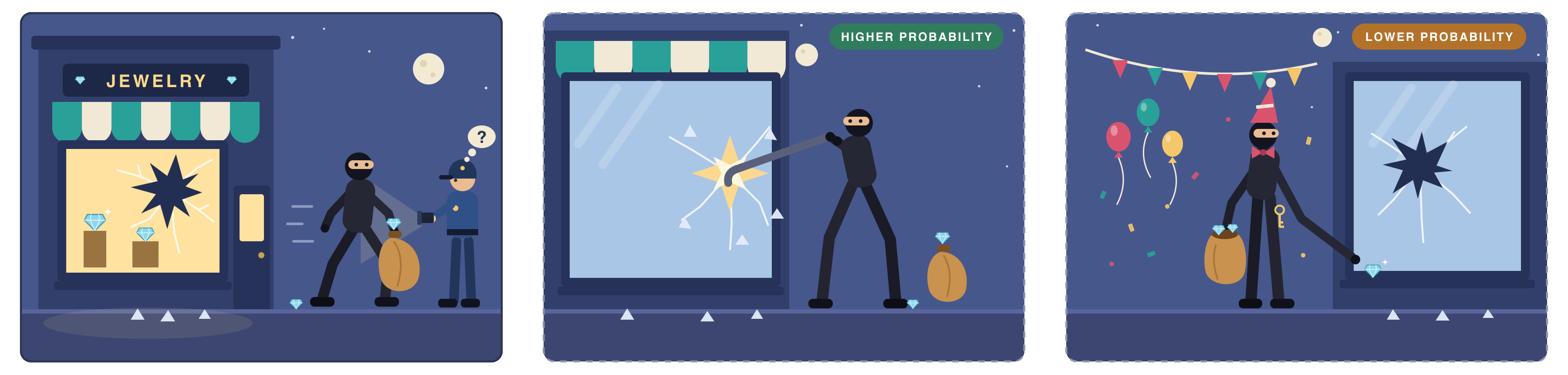
A person with mask is take a bag with some diamonds and walk out of a jewelry store with broken windows. The police will naturally assume that the person is a thief. But it is possible that the person is a jewelry store owner who just attended a costume party, found the windows were broken and tried to take those diamonds to protect them from being stolen (Jaynes 2021).
Can we say the first assumption is more likely to be true than the second one? Yes, because it is simpler and more consistent with our previous observations and polices’ prior experience. Using a more rigorous way to describe this, we can say that the first assumption has a higher probability.
7.2 Probability
You may heard that the hundred-year aurora and you will say “it is so lucky to see it in my lifetime”. But what does it really mean?
| 1/100 as | 1/100 as |
|---|---|
| the probability of seeing the aurora in a given year | a person’s believe that they will see the aurora in a given year |
Probability is both subjective belief and objective mathematical concept. With probability, we can quantify the uncertainty of induction and say that the probability of the sun rising in the east and all apples falling from trees are closed to 100% based on years of observations. And we can live with the uncertainty of induction, because we can always update our conclusions as new observations and data arrive.
7.3 Sample Space and Events
Consider a situation whose outcome is not yet determined: one year of weather in Seattle, one household’s next five years, your GPA of this class. The sample space \(S\) is the set of EVERY possible outcomes that could occur for a particular question (or situation). An event is any subset of sample space \(S\). A probability is a rule \(P\) attaching a number to each event. For example, \(P(A)\) be the probability of event \(A\).
Example 7.1 Toss a fair coin twice and report if it lands heads or tails.
Sample space: \(\{HH, HT, TH, TT\}\)
Probability: \(P(HH) = P(HT) = P(TH) = P(TT) = 1/4\)
Events: any subset of the sample space, e.g., \(A\text{ (first toss is head)} = \{\text{HH}, \text{HT}\}\), \(B\text{ (getting exactly one head)} = \{\text{HT}, \text{TH}\}\), \(C\text{ (getting 2 heads)} = \{\text{HH}\}\), \(D\text{ (getting at least one head)} = \{\text{HT}, \text{TH}\, \text{HH}\}\).
Events combine in three ways:
- “Not \(A\)” is the complement \(A^c\), the outcomes in \(S\) not in \(A\).
- “\(A\) or \(B\)” is the union \(A \cup B\), the outcomes in at least one.
- “\(A\) and \(B\)” is the intersection \(A \cap B\), the outcomes in both.
- Two events are mutually exclusive when they cannot both happen, so \(A \cap B\) is empty \(\emptyset\).
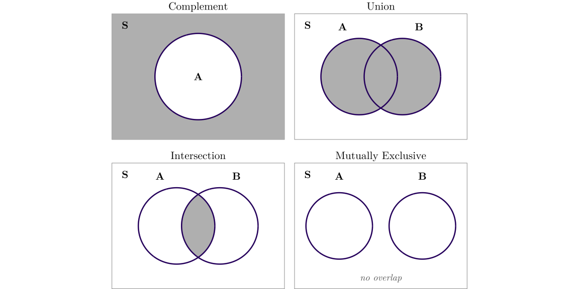
Let \(A\) and \(B\) be two events, \(P(A)\) and \(P(B)\) be their probabilities. The following rules always hold:
- \(0 \le P(A) \le 1\)
- \(P(S) = 1\)
- \(P(A^C) = 1 - P(A)\)
- \(P(A \cup B) = P(A) + P(B) - P(A \cap B)\)
Example 7.2 A flood has a 1% chance of happening in any given year, and a flood this year does not change next year’s chance. What is the chance of at least one flood in the next 10 years?
Multiplying gives \(10 \times 1\% = 10\%\), and 100 years would make a flood certain, which is intuitively incorrect. No flood in one year has probability \(0.99\). No flood in 10 years means none in year 1, none in year 2, and so on, so with the years independent it is \(0.99^{10} = 0.904\). At least one flood is everything else:
\[P(\text{at least one flood in } n \text{ years}) = 1 - 0.99^{\,n}\]
| Years n | Chance of at least one flood (%) | Average number of floods |
|---|---|---|
| 1 | 1.0 | 0.01 |
| 10 | 9.6 | 0.10 |
| 30 | 26.0 | 0.30 |
| 50 | 39.5 | 0.50 |
| 100 | 63.4 | 1.00 |
7.4 Conditional Probability
The conditional probability of \(A\) given \(B\) is the probability of \(A\) when we know that \(B\) has occurred:
\[P(A \mid B) = \frac{P(A \cap B)}{P(B)}, \qquad P(B) > 0.\]
Rearranged, this is the multiplication rule \(P(A \cap B) = P(A \mid B)\,P(B)\).
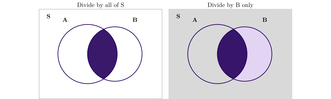
Example 7.3 Toss a fair coin twice, as in Example 7.1. If we know that at least one toss landed heads (event \(D\)), what is the probability that both landed heads (event \(C\))?
\[P(C \mid D) = \frac{P(C \cap D)}{P(D)} = \frac{1/4}{3/4} = \frac{1}{3}.\]
7.5 Independence
Events \(A\) and \(B\) are independent when knowing \(B\) does not change the probability of \(A\), that is, \(P(A \mid B) = P(A)\). Therefore, when \(A\) and \(B\) are independent, \(P(A \cap B) = P(A)\,P(B)\).
Example 7.4 Suppose a plan puts the annual chance of a damaging earthquake at 5% and of a damaging landslide at 3%. Multiplying gives 0.15% for both, but earthquakes trigger landslides, so \(P(\text{landslide} \mid \text{earthquake})\) is far larger than 3%, and the correct joint probability is \(P(\text{earthquake}) \times P(\text{landslide} \mid \text{earthquake})\). When hazards reinforce one another, assuming independence understates the joint probability, so multi-hazard analyses that assume it come out optimistic.
7.6 Law of Total Probability
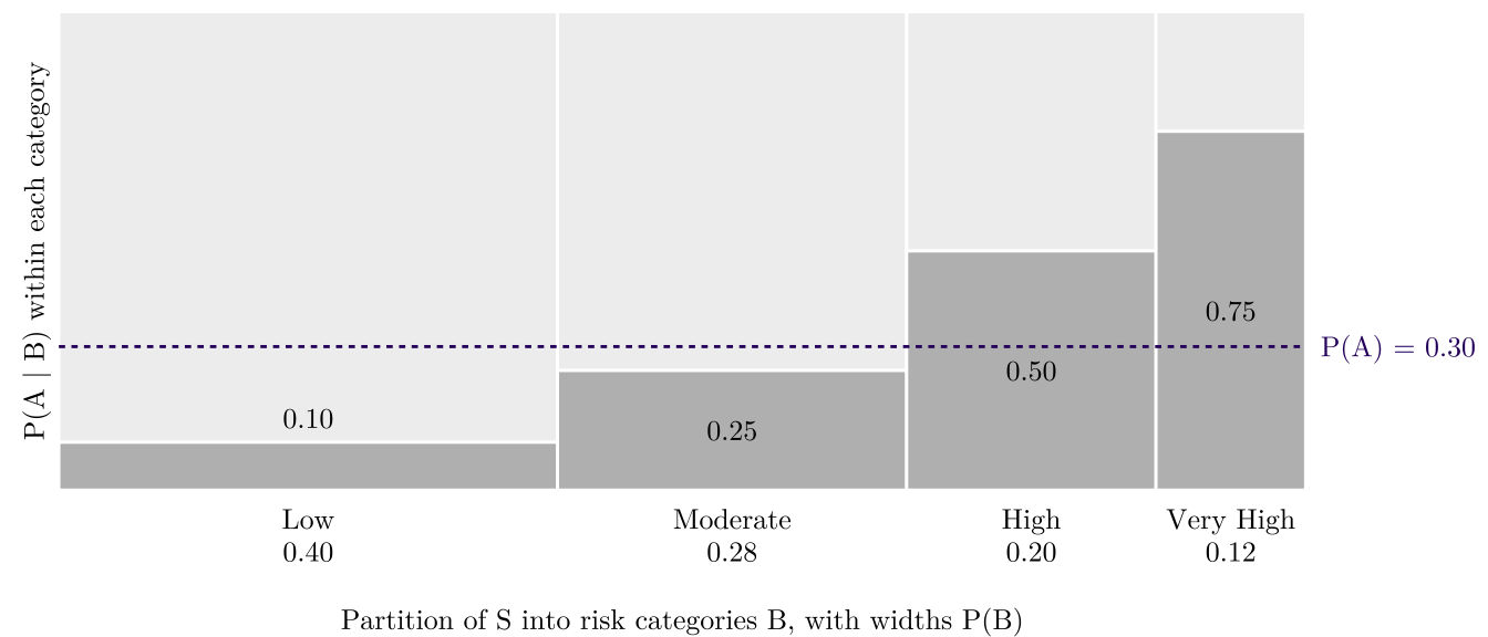
When events \(B_1, \dots, B_k\) are mutually exclusive and together exhaust \(S\) — a partition, such as the risk categories of a classified map — the law of total probability gives
\[P(A) = \sum_{i=1}^{k} P(A \mid B_i)\,P(B_i),\]
7.7 Bayes’ Rule
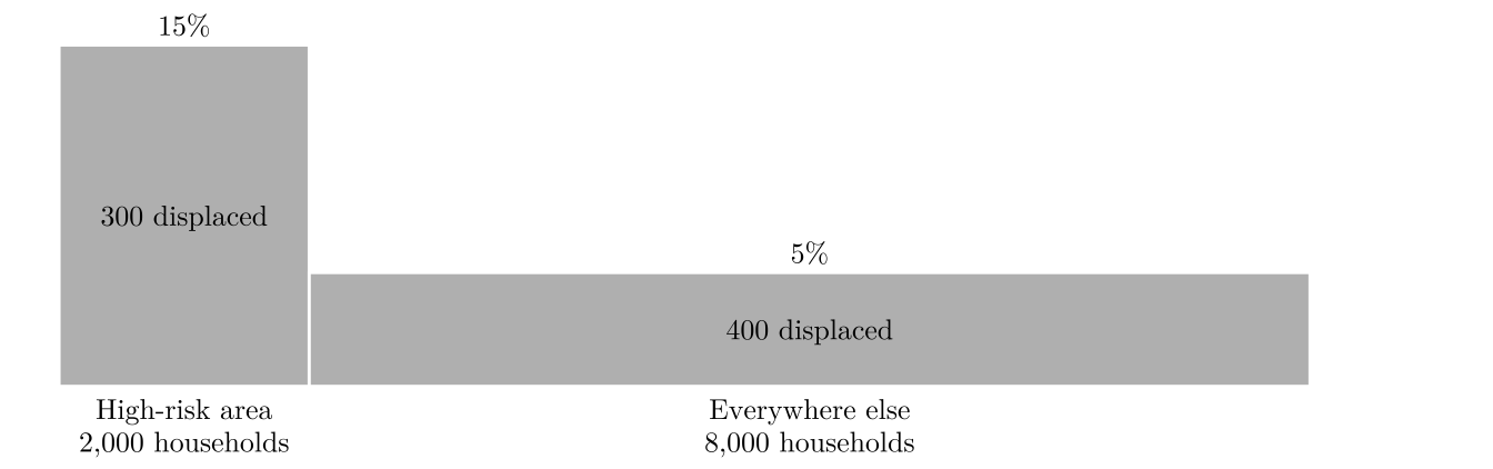
A conditional probability and its reverse are different quantities. Take 10,000 low-income renter households. Over five years, 15% households in a high-risk area are displaced, against 5% elsewhere. You may have the conclusion that if we randomly select a displaced household, it is more likely to be from the high-risk area. But if we consider the total households in both areas, this household is more likely to be from everywhere else!
| Displaced | Not displaced | Total | |
|---|---|---|---|
| High-risk area | 300 | 1,700 | 2,000 |
| Everywhere else | 400 | 7,600 | 8,000 |
| Total | 700 | 9,300 | 10,000 |
Reading across the first row: 300 of 2,000, so \(P(\text{displaced} \mid \text{high risk}) = 0.15\), against 0.05 elsewhere. Reading down the first column: 300 of 700, so \(P(\text{high risk} \mid \text{displaced}) = 0.43\). Most displaced households were not in the high-risk area. A program that spends only inside the high-risk area misses over half of the displaced households (Figure 7.6).
Bayes’ rule expresses the same computation. Substituting the multiplication rule into the definition of conditional probability, with the law of total probability supplying the denominator:
\[P(B \mid A) = \frac{P(A \mid B)\,P(B)}{P(A)} = \frac{P(A \mid B)\,P(B)}{P(A \mid B)\,P(B) + P(A \mid B^c)\,P(B^c)}\]
It is important to remember that \(P(A\mid B)\) and \(P(B\mid A)\) have different meanings. And Bayes’ rule tells us how to invert conditional probabilities from one to another.
Example 7.5 Let’s consider a classical example of Bayes’ rule. Suppose a disease affects 1% of the population. A test for the disease is 99% accurate, meaning that it correctly identifies 99% of those with the disease (we call true positives) and correctly identifies 99% of those without the disease (true negatives). If a person tests positive, what is the probability that they actually have the disease?
Translating this into probabilities: \(P(\text{disease}) = 0.01\), \(P(\text{test positive} \mid \text{disease}) = 0.99\), \(P(\text{test negative} \mid \text{no disease}) = 0.99\)); we want to find \(P(\text{disease} \mid \text{test positive})\). Based on total law of probability and Bayes’ rule, we have:
\[ \begin{aligned} P(\text{test positive}) &= P(\text{test positive} \mid \text{disease})\,P(\text{disease}) + P(\text{test positive} \mid \text{no disease})\,P(\text{no disease}) \\ &= 0.99 \times 0.01 + 0.01 \times 0.99 \\ &= 0.0198 \\[1em] P(\text{disease} \mid \text{test positive}) &= \frac{P(\text{test positive} \mid \text{disease})\,P(\text{disease})}{P(\text{test positive})} \\ &= \frac{0.99 \times 0.01}{0.0198} \\ &= 0.5 \end{aligned} \]
We can also make a table to illustrate. Assume that out of 10,000 people:
| Category | Test Positive | Test Negative | Total |
|---|---|---|---|
| Disease | 99 | 1 | 100 (1%) |
| No Disease | 99 | 9,801 | 9,900 (99%) |
| Total | 198 | 9,802 | 10,000 (100%) |
When people tell you that the test is 99% accurate, the probability they are referring to is \(P(\text{test positive} \mid \text{disease})\). However, the probability of actually having the disease given a positive test result, \(P(\text{disease} \mid \text{test positive})\), is the thing people really care about.
Figure 7.7 draws the 10,000 people of Table 7.4 as squares, for other shares with the disease and other accuracies. At 99% accuracy, \(P(\text{disease} \mid \text{test positive})\) falls to 0.09 when 1 person in 1,000 has the disease and rises to 0.92 when 1 in 10 does.
7.7.1 Bayesian Way of Thinking
Bayes’ rule is simply in its format but profound in its implications and philosophy significance. The formula exactly shows how to update our beliefs in light of new evidence:
\[\underbrace{P(H \mid E)}_{\text{Posterior: Updated Belief}} = \underbrace{P(H)}_{\text{Prior: Existing Knowledge}} \times \underbrace{\frac{P(E \mid H)}{P(E)}}_{\text{Update Factor: Impact of Evidence}}\]
Prior knowledge (\(P(H)\)) is what we already know. After getting new evidences (\(E\)), we update our belief to get the posterior probability (\(P(H \mid E)\)). The update factor \(\frac{P(E \mid H)}{P(E)}\) tells us how much the new evidence should change our belief. For example, if the evidence is very likely given the prior knowledge, then it will increase our belief in the hypothesis.
Example 7.6 Imagine you are looking for a standing desk on Amazon. You find a product with a perfect 5.0-star rating, but it only has 3 reviews. How do you think about the rate? Will you purchase it? What about a desk with a 4.8-star rating after 3,000 reviews?
7.8 Two Readings of a Probability
There are two primary interpretations of probability. Under the frequentist interpretation, \(P(A)\) (e.g., the probability of a coin landing heads) is an unknown but fixed parameter of the population. We estimate it based on samples (recall Figure 2.1). One estimator for \(P(A)\) is the relative frequency of \(A\) occurring over many repeated coin tosses.
Under the Bayesian interpretation, \(P(A)\) measures the degree of belief: how strongly a person expects \(A\) to occur given their current knowledge. For a coin toss, before seeing any data, we might assign \(P(A)\) a prior probability of 0.5. As we toss the coin and gather new data, we use Bayes’ theorem to update this into a posterior probability. In this process, \(P(A)\) is not a fixed parameter, but a variables that updates our belief as new evidence comes.