8 Probability Distributions
I can’t tell you the details of the Gaussian distribution, but I know what it looks like and I know that many events and phenomena in real life are distributed that way.
Charlie Munger
8.1 Random Variables
A random variable (RV) assigns a number to each outcome of a chance process. If \(X\) is the number of rainy days in Seattle next year, \(X\) could be 180, 250, or 365. Before the year runs, which value of \(X\) is random1. We use \(P(X=x)\) to represent the probability that the RV \(X\) will be a constant number \(x\).
1 Formally a random variable is a function from the sample space to the real numbers. Capital letters name random variables and lower case letters name their realized values, so \(P(X = 365)\) is the probability of a year with rain every day, and \(x = 214\) is what a particular year delivered.
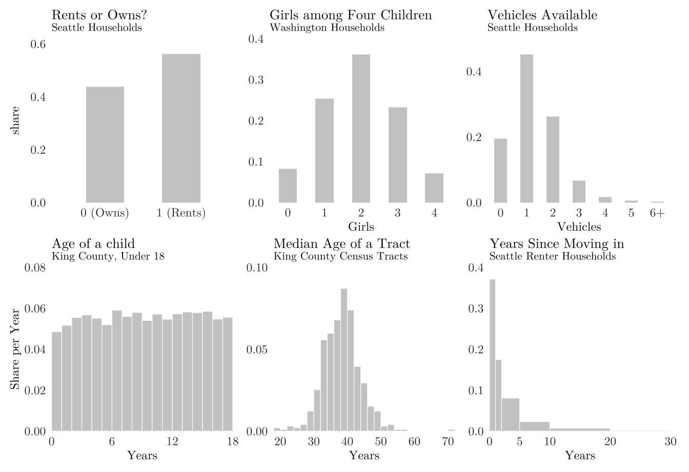
Random variable can take different types of values. A random variable is discrete when its possible values can be listed, with gaps between them, such as housing units on a parcel or vehicles in a household. It is continuous when it can take any value in an interval, such as parcel area or construction cost. The following figure shows six values from the American Community Survey.
Example 8.1 Seattle Department of Transportation wants to know the true average daily walking steps of all residents to fund a new sidewalk expansion. They randomly sample 50 residents every week and calculate the average steps. Is the weekly sample mean \(\bar X\) a constant or a random variable?
8.2 Discrete Random Variables
For a discrete variable the distribution can be written out by probability mass function (PMF): \[p(x) = P(X = x), \quad 0 \le p(x) \le 1 \ \text{ for every } x, \quad \sum_{x} p(x) = 1\]
Example 8.2 Let \(X\) be the number of vehicles available to a randomly chosen household in an urban tract, with shares rounded to two decimals:
| \(x\) vehicles | 0 | 1 | 2 | 3 | 4 |
|---|---|---|---|---|---|
| \(p(x)\) | 0.12 | 0.38 | 0.35 | 0.11 | 0.04 |
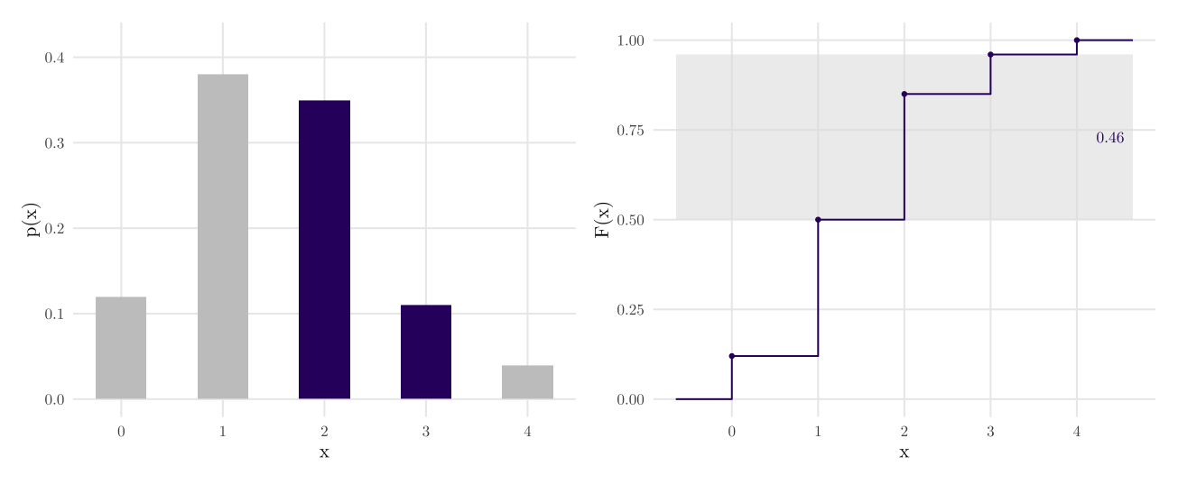
The five probabilities sum to 1. The share of households with no car is \(p(0) = p(X=0) = 0.12\). The share with at least one is \(1 - p(0) = 0.88\). The share with two or more is \(p(2) + p(3) + p(4) = 0.50\).
8.2.1 Cumulative Distribution Function
The cumulative distribution function (CDF) accumulates that probability that:
\[F(x) = P(X \le x) = \sum_{t \le x} p(t), \quad P(X > a) = 1 - F(a)\]
Every distribution has a CDF, discrete or continuous, and the CDF determines the distribution completely. It starts at 0, ends at 1, and never decreases.
8.3 Expectation and Standard Deviation
A distribution has a center and a spread, which are similar to the mean and SD we saw before, but computed from probabilities instead of observations/data. The expectation is the expected value of a random variable. For a discrete variable, it is the probability-weighted average of the values:
\[\mu = E[X] = \sum_{x} x\,p(x)\]
The variance is the probability-weighted average squared distance from that expectation, and the standard deviation is its square root:
\[\sigma^2 = \operatorname{Var}(X) = \sum_{x} (x - \mu)^2 p(x), \quad \sigma = \sqrt{\sigma^2}\]
For Table 8.1, we can calculate expectation and variance as:
\[\begin{aligned} \mu &= 0(0.12) + 1(0.38) + 2(0.35) + 3(0.11) + 4(0.04) = 1.57 \\ \sigma^2 &= (0 - 1.57)^2(0.12) + (1 - 1.57)^2(0.38) + (2 - 1.57)^2(0.35) \\ &\quad + (3 - 1.57)^2(0.11) + (4 - 1.57)^2(0.04) = 0.945 \end{aligned}\]
8.3.1 Features of Expectation and Variance
Note here, we use Greek letters \(\mu\) and \(\sigma\), which are the same as the symbols used to denote the population mean and population standard deviation. This notation emphasizes that the center and spread of a theoretical probability distribution represent the true parameters of the underlying system, rather than temporary statistics calculated from a limited sample of observed data.
Three rules cover almost every calculation about expectation and variance. For constants \(a\) and \(b\),
\[E[aX + b] = a\,E[X] + b, \qquad \operatorname{SD}(aX + b) = |a|\operatorname{SD}(X),\]
For any two random variables, expected values add: \(E[X + Y] = E[X] + E[Y]\), whether or not \(X\) and \(Y\) are related. Variances add only under independence:
\[\operatorname{Var}(X + Y) = \operatorname{Var}(X) + \operatorname{Var}(Y) \quad \text{when } X \text{ and } Y \text{ are independent.}\]
Standard deviations never add. Two independent RVs with SDs of \(\$30,000\) each give a total SD of \(\sqrt{30{,}000^2 + 30{,}000^2} \approx \$42{,}400\).
8.4 Common Discrete Distributions
Writing a distribution out value by value works for 5 values, like Table 8.1, and not for 5000 values. We have some named distributions with a few parameters. Those distributions can wonderfully describe some common processes.
8.4.1 Bernoulli: One Trial
A Bernoulli variable is a single trial with two outcomes, 1 or 0, yes or no. Its only parameter is \(p\), which means the probability of getting 1. If a random variable \(X\) follow Bernoulli distribution, we write as \(X \sim \text{Ber}(p)\):
\[P(X = 1) = p, \qquad P(X = 0) = 1 - p, \qquad E[X] = p, \qquad \operatorname{Var}(X) = p(1 - p)\]
8.4.2 Binomial: Successes in Trials
Add up \(n\) independent Bernoulli trials with the same \(p\) and the total is binomial, written \(X \sim \text{Bin}(n, p)\). Then the PMF of \(X \sim \text{Bin}(n, p)\) is:
\[P(X = k) = \binom{n}{k} p^{k} (1-p)^{n-k}, \quad k = 0, 1, \dots, n,\]
\[E[X] = np, \quad \operatorname{Var}(X) = np(1-p), \quad \operatorname{SD}(X) = \sqrt{np(1-p)}.\]
The binomial coefficient \(\binom{n}{k} = \frac{n!}{k!\,(n-k)!}\) counts the orderings: there are \(\binom{n}{k}\) different ways for \(k\) of \(n\) trials to succeed (we call combination), and \(p^k(1-p)^{n-k}\) is the probability of any one of them.
Example 8.3 Based on inspection records to privately owned stormwater facilities, 80 percent of sites stay in compliance for at least two years (Stormwater Management Program Plan 2026). Inspectors return to 20 sites two years after their last inspection. If each site is compliant with probability 0.8, independently of the others, the number found compliant is \(X \sim \text{Bin}(20, 0.8)\):
\[E[X] = 20(0.8) = 16, \quad \operatorname{SD}(X) = \sqrt{20(0.8)(0.2)} = 1.79\]
The probability that exactly 16 are compliant is \(P(X=16)=\binom{20}{16}(0.8)^{16}(0.2)^{4} = 0.218\).
8.4.3 Poisson: Counts in a Window
The Poisson distribution counts events in a fixed window of time or space, such as the number of accidents at an intersect in a month, number of demolition permits in a neighborhood in a year. Poisson distribution only has one parameter \(\lambda\), which is both the mean and variance of the distribution. Then the PMF of \(X \sim \text{Pois}(\lambda)\) is:
\[P(X = k) = \frac{\lambda^{k} e^{-\lambda}}{k!}, \qquad k = 0, 1, 2, \dots\]
\[E[X] = \lambda, \quad \operatorname{Var}(X) = \lambda, \quad \operatorname{SD}(X) = \sqrt{\lambda}\]
Example 8.4 In parts of Seattle, stormwater and sewage share one pipe, and a heavy storm can overflow it into nearby water. Washington allows each overflow point an average of one untreated discharge per year based on WAC 173-245-020(22). Take an outfall that meets the rule and its number of overflows in a year is \(X \sim \text{Pois}(1)\), with \(E[X] = 1\) and \(\operatorname{SD}(X) = 1\).
\[P(X = 0) = e^{-1} = 0.368, \quad P(X = 1) = e^{-1} = 0.368, \quad P(X \ge 2) = 1 - 0.368 - 0.368 = 0.264\]
An outfall that meets the rule still have 26.4% probability that overflows two or more times in a year.
8.4.4 Comparing the Three
| Distribution | The story | \(P(X=k)\) | \(E[X]\) | \(\operatorname{Var}(X)\) | R |
|---|---|---|---|---|---|
| Bernoulli(\(p\)) | one trial, two outcomes | \(p^k(1-p)^{1-k}\) | \(p\) | \(p(1-p)\) | dbinom |
| Binomial(\(n,p\)) | successes in \(n\) fixed independent trials | \(\binom{n}{k}p^k(1-p)^{n-k}\) | \(np\) | \(np(1-p)\) | dbinom |
| Poisson(\(\lambda\)) | events in a fixed window, no denominator | \(\lambda^k e^{-\lambda}/k!\) | \(\lambda\) | \(\lambda\) | dpois |
d for the mass function, p for the CDF, q for the quantile, r for random draws, so dbinom, pbinom, qbinom, rbinom.
Try to set the binomial to \(n = 40\), \(p = 0.5\) and watch the shape become symmetric and bell-like. There are more discrete distributions but we will not cover here, such as geometric distribution and negative binomial distribution.
8.5 Continuous Random Variables
A continuous random variable can take any value in an interval. There are infinitely many such values, so the probability of any one exact value is 0, \(P(X = x) = 0\), and probability is assigned to intervals instead. The probability density function (PDF) \(f(x)\) is the continuous version of PMF and the probability of an interval is the area under \(f(x)\) over that interval.
\[P(a \le X \le b) = \int_{a}^{b} f(x)\,dx, \quad f(x) \ge 0, \quad \int_{-\infty}^{\infty} f(x)\,dx = 1\]
The CDF is the same as before, \(F(x) = P(X \le x)\), and \(P(a \le X \le b) = F(b) - F(a)\).
Recall the figure in lecture 1. The PDF and the CDF are the pair: CDF \(F(x_0)\) is the area under PDF \(f\) up to \(x_0\), and \(f(x_0)\) is the slope of \(F\) at \(x_0\).
8.5.1 From Histogram to Density
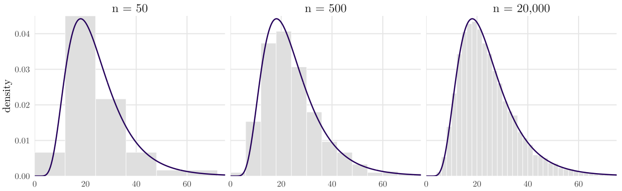
A density is what a histogram becomes with more data and narrower bins. A histogram describes a sample; a density describes the population the sample came from.
8.5.2 Expectation and Variance
The definitions are the same as for a discrete variable, with the sum replaced by an integral and the probability \(p(x)\) by the density \(f(x)\):
\[\mu = E[X] = \int_{-\infty}^{\infty} x\,f(x)\,dx\]
\[\sigma^2 = \operatorname{Var}(X) = \int_{-\infty}^{\infty} (x - \mu)^2 f(x)\,dx = E[X^2] - \mu^2, \quad \sigma = \sqrt{\sigma^2}\]
The rules in Features of Expectation and Variance hold for continuous variables as well.
8.6 Common Continuous Distributions
8.6.1 Uniform
A uniform variable is equally likely to fall anywhere in an interval \([a, b]\), written \(X \sim \text{Unif}(a, b)\):
\[f(x) = \frac{1}{b-a} \ \text{ for } a \le x \le b, \quad F(x) = \frac{x-a}{b-a}, \quad E[X] = \frac{a+b}{2}, \quad \operatorname{Var}(X) = \frac{(b-a)^2}{12}\]
Example 8.5 SDOT has improved its street-tree pruning cycle to nine years (Urban Forest Management Plan 2020). If SDOT works through the trees evenly, the time since a randomly chosen street tree was last pruned is \(X \sim \text{Unif}(0, 9)\) years:
\[E[X] = \frac{0 + 9}{2} = 4.5, \quad \operatorname{SD}(X) = \frac{9}{\sqrt{12}} = 2.6, \quad P(X > 6) = \frac{9 - 6}{9} = 0.33\]
8.6.2 Normal/Gaussian
A normal or Gaussian variable, written \(X \sim N(\mu, \sigma^2)\), has a symmetric, bell-shaped density:
\[f(x) = \frac{1}{\sigma\sqrt{2\pi}}\exp\!\left(-\frac{(x-\mu)^2}{2\sigma^2}\right), \quad E[X] = \mu, \quad \operatorname{Var}(X) = \sigma^2\]
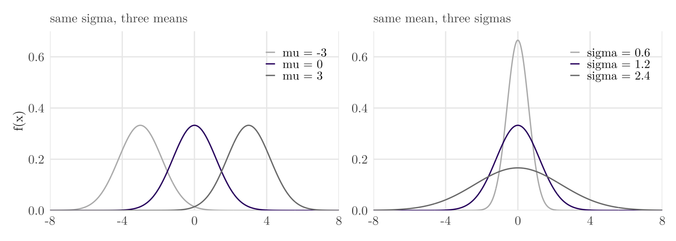
\(\mu\) moves the curve along the axis and \(\sigma\) sets its spread. Because the area under the curve is always 1, a larger \(\sigma\) gives a lower peak.
The empirical rule: for any normal variable, about 68 percent of the probability lies within one \(\sigma\) of \(\mu\), 95 percent within two, and 99.7 percent within three.
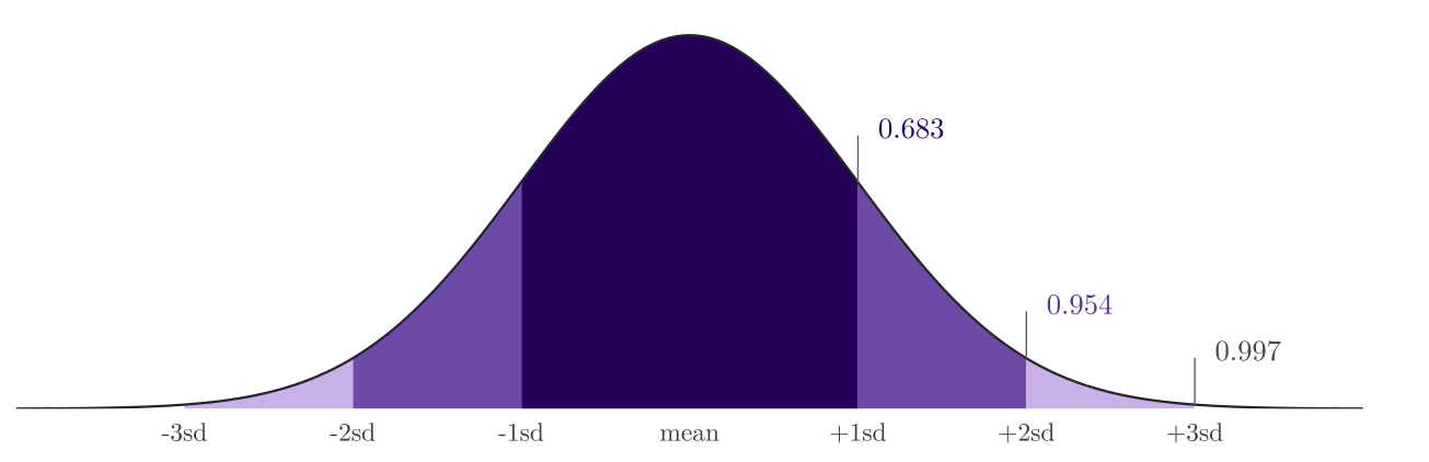
Any normal variable becomes the standard normal \(Z\) by subtracting its mean and dividing by its standard deviation. This is the z-score in standardization:
\[Z = \frac{X - \mu}{\sigma} \sim N(0, 1)\]
Example 8.6 Suppose that peak-period travel time on a corridor is \(X \sim N(28, 8^2)\) minutes.
A 44-minute trip is two SDs above the mean: \(z = (44 - 28)/8 = 2\). About 95 percent of trips lie within two SDs, and the other 5 percent split evenly between the two tails, so \(P(X > 44) \approx 0.05/2 = 0.025\).
About 68 percent of trips take between \(20\) and \(36\) minutes, within one SD. Half of the other 32 percent take longer than 36 minutes, so 36 minutes covers about \(68 + 16 = 84\) percent of trips.
Example 8.7 King County home prices in 2025 are right-skewed, and the empirical rule fails on them: 89.1% of the 16,113 sales lie within one SD of the mean price. Their natural logarithms are close to normal, with mean 13.85 and SD 0.512, and for the standardized log price \(Z\):
\[P(|Z| < 1) = 0.692, \qquad P(|Z| < 2) = 0.962, \qquad P(|Z| < 3) = 0.995\]
8.6.2.1 Properties of Normal Random Variables
Linear combinations. If \(X \sim N(\mu_X, \sigma_X^2)\) and \(Y \sim N(\mu_Y, \sigma_Y^2)\) are independent and \(a\), \(b\) and \(c\) are all constants, then
\[aX \pm bY + c \sim N\!\left(a\mu_X \pm b\mu_Y + c,\ a^2\sigma_X^2 + b^2\sigma_Y^2\right).\]
Notice that \(X-Y\) has variance \(\sigma_X^2 + \sigma_Y^2\), not \(\sigma_X^2 - \sigma_Y^2\).
Example 8.8 Suppose, for the arithmetic, that a household’s monthly rent is \(R \sim N(1800, 200^2)\) dollars and its utilities, independent of the rent, are \(U \sim N(150, 40^2)\). The monthly housing cost is
\[R + U \sim N(1950,\ 200^2 + 40^2), \quad \operatorname{SD} = \sqrt{41{,}600} = 204,\]
8.6.2.2 Chi-square Distribution
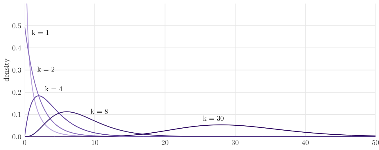
The chi-square distribution. If \(Z_1, \dots, Z_k\) are independent standard normal variables \(N(0,1)\), the sum of their squares has the chi-square distribution with \(k\) degrees of freedom:
\[Q = Z_1^2 + Z_2^2 + \cdots + Z_k^2 \sim \chi^2_k, \quad E[Q] = k, \quad \operatorname{Var}(Q) = 2k.\]
As \(k\) grows it moves right and, being a sum of independent terms, becomes more symmetric.
8.6.3 Exponential: Wait Between Events
An exponential variable, written \(X \sim \text{Exp}(\lambda)\), is the waiting time until the next event when events happen at a constant rate \(\lambda\):
\[f(x) = \lambda e^{-\lambda x}, \quad F(x) = 1 - e^{-\lambda x} \ (x \ge 0), \quad E[X] = \frac{1}{\lambda}, \quad \operatorname{Var}(X) = \frac{1}{\lambda^{2}}\]
\(\lambda\) is a rate, so the mean wait is \(1/\lambda\): 6 events per hour means a mean wait of 10 minutes. The exponential is the Poisson seen from the other side: if the number of events in a window is \(\text{Pois}(\lambda)\), the time between events is \(\text{Exp}(\lambda)\).
Example 8.9 The outfall in Example 8.4 overflows at a rate of \(\lambda = 1\) per year, so the time \(T\) until its next overflow is \(T \sim \text{Exp}(1)\), with a mean of 1 year.
\[P(T > 2) = e^{-2} = 0.135, \quad P(T \le 0.5) = 1 - e^{-0.5} = 0.393\]
8.6.4 Comparing the Three
| Distribution | The story | \(f(x)\) | \(E[X]\) | \(\operatorname{Var}(X)\) | R |
|---|---|---|---|---|---|
| Uniform(\(a,b\)) | flat over an interval; often an assumed range | \(1/(b-a)\) | \((a+b)/2\) | \((b-a)^2/12\) | dunif |
| Normal(\(\mu,\sigma^2\)) | symmetric; sums and averages of many small effects | see above | \(\mu\) | \(\sigma^2\) | dnorm |
| Exponential(\(\lambda\)) | wait until the next event at constant rate \(\lambda\) | \(\lambda e^{-\lambda x}\) | \(1/\lambda\) | \(1/\lambda^2\) | dexp |
The panel below draws the three continuous distributions. Beyond the three, there are more common continuous distributions, such as gamma distributions and beta distributions.