14 Linear Regression
All models are wrong, but some are useful.
George Box
14.1 Predicting by Guessing
To predict a value we do not know, we start from what we do know. Table 14.1 lists my guesses of a housing index for five metropolitan areas, made from their population and other known data.
| Region | Population | Other Info | My Guess Index | Real Housing Index |
|---|---|---|---|---|
| New York, NY | 19,940,274 | … | 22000 | 22000 |
| Los Angeles, CA | 12,927,614 | … | 19000 | 22200 |
| Chicago, IL | 9,408,576 | … | 17000 | 15600 |
| Dallas, TX | 8,344,032 | … | 10000 | 12900 |
| Houston, TX | 7,796,182 | … | 11000 | 12400 |
The guesses are inaccurate: some guesses are close and some are far off. In order to compare ways of guessing, we first need to define what a good guess is.
14.1.1 Mean Squared Error
Write \(Y_i\) for the real/observed value of observation \(i\) and \(\hat{Y}_i\) for the guess. The prediction error of observation \(i\) is \(Y_i - \hat{Y}_i\). The mean absolute error (MAE) is the average size of the prediction errors, and the mean squared error (MSE)1 is the average of their squares:
1 The MSE here is computed from one set of data and one particular model. The MSE in estimation belongs to an estimator: the average of \((\hat\theta - \theta)^2\) over all possible samples.
\[\text{MAE} = \frac{1}{n}\sum_{i=1}^{n}\left|Y_i - \hat{Y}_i\right|, \quad \text{MSE} = \frac{1}{n}\sum_{i=1}^{n}\left(Y_i - \hat{Y}_i\right)^2\]
The MSE is in squared units of \(Y\). Its square root, the root mean squared error (RMSE), is in the units of \(Y\). The MSE is just one way to define the error of a prediction, and the usual one in regression.
Example 14.1 In Table 14.1, the real index minus the guess is \(0\), \(3200\), \(-1400\), \(2900\), and \(1400\).
\[\text{MAE} = \frac{0 + 3200 + 1400 + 2900 + 1400}{5} = 1780\]
\[\text{MSE} = \frac{0^2 + 3200^2 + 1400^2 + 2900^2 + 1400^2}{5} = 4514000\]
The RMSE is \(\sqrt{4,514,000} \approx 2,125\) index points. It is larger than the MAE, because the two large misses weigh more after squaring.
14.1.2 Best MSE Predictors
If we wish to predict the \(y\) without any known information beyond \(y\), the best guess is the same guess \(c\) for every observation. For any \(c\) in terms of MSE:
\[MSE = \frac{1}{n}\sum_{i=1}^{n}(Y_i - c)^2 = \frac{1}{n}\sum_{i=1}^{n}(Y_i - \bar{Y})^2 + (\bar{Y} - c)^2\]
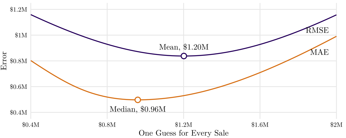
The first term does not depend on \(c\), so the MSE is smallest at \(c = \bar{Y}\). In terms of MSE, the best single guess is the mean, and its MSE is the variance of \(Y\) (with \(n\) in the denominator). In terms of MAE, the best single guess is the median (proof skipped).
Example 14.2 Guessing the mean price ($1,201,401) for every one of the King County sales of 2025 gives an RMSE of about $838,000. Guessing the median ($960,000) gives a larger RMSE, $872,000, but a smaller MAE: $497,000 against $530,000.
With known data \(X\), we can guess differently for different observations. The conditional expectation \(E[Y \mid X = x]\) is the mean of \(Y\) among the observations with \(X = x\). Given the known data \(X\), the conditional expectation has the smallest MSE of all predictors:
\[\text{Best MSE Predictor} = E[Y \mid X]\]
Example 14.3 The mean price of the King County sales is $811,000 with 2 bedrooms, $1,014,000 with 3, and $1,373,000 with 4. Guessing the mean of its bedroom count for each sale, instead of the overall mean, lowers the RMSE from $838,000 to $782,000.
14.2 What is Linear Regression
\(E[Y \mid X]\) needs a separate mean at every possible value of \(X\). That is too ambitious:
- Many values. For example, the King County sales have 863 different living areas, and 345 of them belong to one sale each, whose mean is that sale’s own price.
- Many variables. By putting living area, year built, and city together, the majority (81%) of the sales are alone in their group.
- New values. There is no mean for a value of \(X\) that the data do not contain.
Linear regression replaces the separate means with a line:
\[E[Y \mid X = x] \approx \beta_0 + \beta_1 x\]
Of all possible lines, we use the one with the smallest MSE. It is called the least squares line, because it makes the sum of the squared prediction errors as small as possible. You can refer to this visualization: Seeing Theory - Ordinary Least Squares.
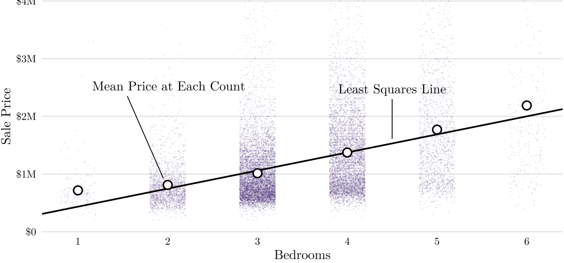
Linear regression is for a continuous \(Y\). Other types of regression handle other response variables, such as logistic (1/0), Poisson (count), and multinomial (categories). With one explanatory variable, the model is a simple linear regression; with several, a multiple linear regression.
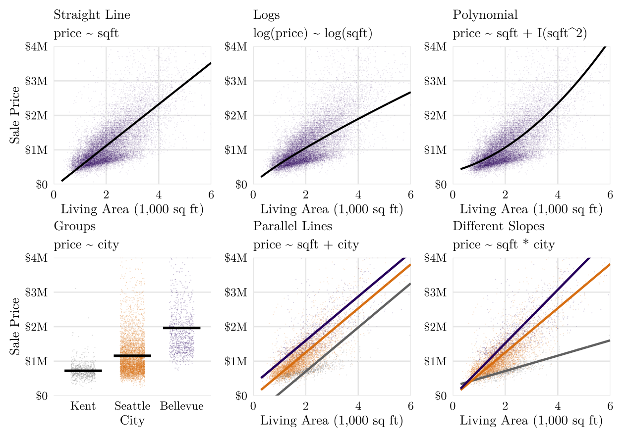
Linear regression is more flexible than a straight line. This figure shows six types of linear regressions.
14.2.1 Common Terms
\[Y_i = \beta_0 + \beta_1 X_{i} + \varepsilon_i\]
- \(Y_i\): the response variable, also called the dependent variable or the outcome
- \(X_i\): the explanatory variables, also called independent variables, predictors, or features
- \(\beta_0\): the intercept
- \(\beta_1, \dots, \beta_k\): the coefficients, or slopes
- \(\varepsilon_i\): the error term, or random, the part of \(Y_i\) that the line does not explain
The \(\beta\)s describe the line in the population. We will never know them. Their estimates from a sample carry a hat, \(\hat\beta\) (sometimes also written \(b\)).
14.2.2 Linear Regression for Prediction
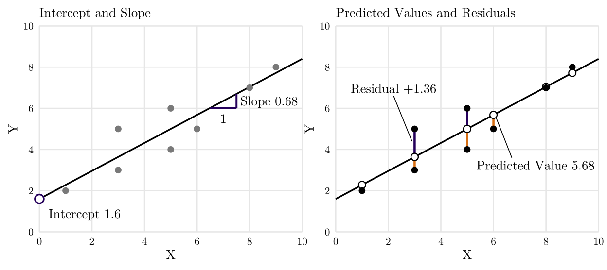
With estimated coefficients, the predicted value (or fitted value) of observation \(i\) is
\[\hat{Y}_i = \hat{\beta}_0 + \hat{\beta}_1 X_{i} \]
The residual of observation \(i\) is its observed value minus its predicted value:
\[e_i = Y_i - \hat{Y}_i\]
14.2.3 Error and Residual
The error \(\varepsilon_i\) is the deviation of an observed value from the true value, \(\beta_0 + \beta_1 X_{1i} + \cdots + \beta_k X_{ki}\). It is part of the model, standing for everything that affects \(Y\) but not in the model, and never observed.
The residual \(e_i\) is the deviation of an observed value from the estimated value. It is computed from the data. The residuals estimate the errors.
14.3 Normal Linear Regression
The normal linear regression model is the classical form of linear regression. It adds assumptions about the errors. Under these assumptions, the t-tests and confidence intervals below are valid.
14.3.1 Assumptions
\[Y_i = \beta_0 + \beta_1 X_{1i} + \cdots + \beta_k X_{ki} + \varepsilon_i, \quad \varepsilon_i \sim N(0, \sigma^2)\]
- Linearity. The mean of \(Y\) changes linearly with each \(X\). A variable can be transformed first, such as \(\log(X)\) or \(X^2\); the model must be linear in the \(\beta\)s.
- Independence. The errors are independent of each other. Grouped, time series, and spatial data are often not independent. We will relax this assumption in a future lecture on correlated data.
- Equal variance (homoscedasticity). The errors have the same variance \(\sigma^2\) at every value of \(X\). We can relax this assumption in the future.
- Normality. The errors follow a normal distribution with mean 0. It is fine for a large sample size because of the central limit theorem (CLT).
- No perfect multicollinearity. No \(X\) is a linear combination of the others, such as a total score that is the sum of part A and part B scores.
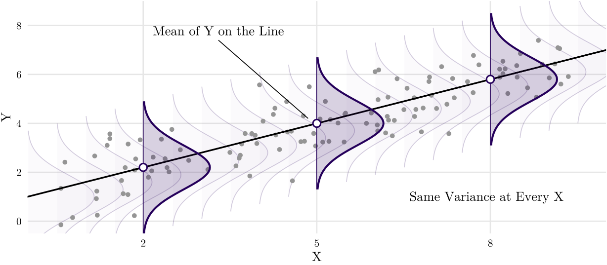
The first four are often remembered as LINE: linearity, independence, normality, equal variance. They are not equally important:
- Linearity matters most. When it fails, the coefficients themselves are wrong: they summarize a non-linear relationship with a line.
- Independence and equal variance do not change the coefficients, only their standard errors, and with them the t-values, p-values, and confidence intervals.
- Without independence, the standard errors are too small, often by a lot.
- Without equal variance, the standard errors can be too small or too large.
- Normality matters least: mostly for the t-tests in small samples.
14.3.2 Covariance Matrix
For \(k\) variables, the covariance matrix \(\mathbf{S}\) lists the covariance of every pair: the entry in row \(j\) and column \(l\) is the covariance \(s_{jl}\) of variables \(j\) and \(l\). The covariance of a variable with itself is its variance, so the diagonal holds the variances:
\[\mathbf{S} = \begin{pmatrix} s_1^2 & s_{12} & \cdots & s_{1k} \\ s_{21} & s_2^2 & \cdots & s_{2k} \\ \vdots & \vdots & \ddots & \vdots \\ s_{k1} & s_{k2} & \cdots & s_k^2 \end{pmatrix}\]
Since \(s_{jl} = s_{lj}\), the matrix is symmetric. In R, cov(d) returns the covariance matrix of the numerical columns of a data frame d.
In regression, the same matrix can describe \(n\) observations \(Y_1, \dots, Y_n\) of one variable, such as the prices of \(n\) sales, each a random variable; the matrix is then \(n\) by \(n\).
- Independent observations with the same variance \(\sigma^2\) have \(\boldsymbol{\Sigma} = \sigma^2\mathbf{I}\) (left), \(\mathbf{I}\) is the identity matrix.
- Two sales on the same block, observations 1 and 2, can covary (right).
\[\begin{pmatrix} \sigma^2 & 0 & 0 \\ 0 & \sigma^2 & 0 \\ 0 & 0 & \sigma^2 \end{pmatrix} \qquad \begin{pmatrix} \sigma^2 & \sigma_{12} & 0 \\ \sigma_{12} & \sigma^2 & 0 \\ 0 & 0 & \sigma^2 \end{pmatrix}\]
Therefore, the assumptions, independence and equal variance, together say that the covariance matrix of the errors \(\varepsilon_1, \dots, \varepsilon_n\) is \(\sigma^2\mathbf{I}\).
14.3.3 Parameters Point Estimation
With one explanatory variable, the model is
\[Y_i = \beta_0 + \beta_1 X_i + \varepsilon_i\]
Every candidate line, with intercept \(\beta_0\) and slope \(\beta_1\), has an MSE:
\[\text{MSE}(\beta_0, \beta_1) = \frac{1}{n}\sum_{i=1}^{n}\left(Y_i - \beta_0 - \beta_1 X_i\right)^2\]
The ordinary least squares (OLS) estimates are the intercept and the slope with the smallest MSE. Setting the partial derivatives with respect to \(\beta_0\) and \(\beta_1\) to 0 gives
\[\hat{\beta}_1 = \frac{\sum (X_i - \bar{X})(Y_i - \bar{Y})}{\sum (X_i - \bar{X})^2}, \qquad \hat{\beta}_0 = \bar{Y} - \hat{\beta}_1 \bar{X}\]
The slope is the covariance of \(X\) and \(Y\) divided by the variance of \(X\).2
2 In R, lm(y ~ x) computes both estimates. Meanwhile, the maximum likelihood method gives the same estimates: with independent normal errors of equal variance, the likelihood is largest where the sum of squared residuals is smallest.
Example 14.4 Eight made-up points, with \(\bar{X} = \bar{Y} = 5\). We can draw a regression line:
| \(X_i\) | 1 | 3 | 3 | 5 | 5 | 6 | 8 | 9 | Sum |
|---|---|---|---|---|---|---|---|---|---|
| \(Y_i\) | 2 | 3 | 5 | 4 | 6 | 5 | 7 | 8 | |
| \(X_i - \bar{X}\) | \(-4\) | \(-2\) | \(-2\) | 0 | 0 | 1 | 3 | 4 | 0 |
| \(Y_i - \bar{Y}\) | \(-3\) | \(-2\) | 0 | \(-1\) | 1 | 0 | 2 | 3 | 0 |
| \((X_i - \bar{X})(Y_i - \bar{Y})\) | 12 | 4 | 0 | 0 | 0 | 0 | 6 | 12 | 34 |
| \((X_i - \bar{X})^2\) | 16 | 4 | 4 | 0 | 0 | 1 | 9 | 16 | 50 |
| \(\hat{Y}_i\) | 2.28 | 3.64 | 3.64 | 5 | 5 | 5.68 | 7.04 | 7.72 | |
| \(e_i = Y_i - \hat{Y}_i\) | \(-0.28\) | \(-0.64\) | 1.36 | \(-1\) | 1 | \(-0.68\) | \(-0.04\) | 0.28 | 0 |
\[\hat\beta_1 = \frac{34}{50} = 0.68, \qquad \hat\beta_0 = 5 - 0.68 \times 5 = 1.6\]
Example 14.5 For the King County sales, \(\bar{X} = 2{,}140\) sq ft and \(\bar{Y} = \$1{,}201{,}401\). The covariance of living area and price is 516.94 million, and the variance of living area is 858,146:
\[\hat\beta_1 = \frac{516{,}940{,}000}{858{,}146} = 602.4, \qquad \hat\beta_0 = 1{,}201{,}401 - 602.4 \times 2{,}140 \approx -87{,}700\]
Sales that differ by one square foot of living area differ by about $602 in price, on average. The predicted price of a 2,000-square-foot house is about $1.12 million. The intercept, a negative price for a house with no living area, lies far outside the data and has no meaning.
14.3.4 Deriving the Estimates
Setting the two partial derivatives of \(\sum (Y_i - \beta_0 - \beta_1 X_i)^2\) to 0 gives the normal equations:
\[\sum_{i=1}^{n}\left(Y_i - \hat\beta_0 - \hat\beta_1 X_i\right) = 0, \qquad \sum_{i=1}^{n} X_i\left(Y_i - \hat\beta_0 - \hat\beta_1 X_i\right) = 0\]
The first equation says that the residuals add up to 0. Divided by \(n\), it gives \(\hat\beta_0 = \bar{Y} - \hat\beta_1 \bar{X}\). Putting this \(\hat\beta_0\) into the second equation and solving gives \(\hat\beta_1\). With \(k\) explanatory variables, the same steps give \(k + 1\) equations, one for each coefficient.
14.3.5 The Slope and the Correlation
The correlation (Pearson’s \(r\)) says how closely the points follow a straight line; the regression line says which line. In terms of \(r\) and the two standard deviations,
\[\hat\beta_1 = r\,\frac{s_Y}{s_X} = \frac{s_{XY}}{s_X s_Y}\cdot\frac{s_Y}{s_X} = \frac{s_{XY}}{s_X^2}\]
where \(s_{XY}\) is the covariance of \(X\) and \(Y\): the same slope as above. So \(r\) is the slope when both variables are in standard units. The slope has units (\(Y\) per unit of \(X\)), while \(r\) has none: \(r\) says how tightly the points follow the line, \(\hat\beta_1\) how steep the line is.3
3 Predicting \(X\) from \(Y\) gives a different line through the same point of averages, with slope \(r\,s_X/s_Y\) in the units of \(X\) per unit of \(Y\).
14.3.6 Why “Regression”
In standard units, the slope of the least squares line is \(r\). From \(\hat\beta_1 = r\,s_Y/s_X\),
\[\frac{\hat{Y} - \bar{Y}}{s_Y} = r \times \frac{X - \bar{X}}{s_X}\]
An observation \(z\) standard deviations from the mean of \(X\) is predicted to lie \(r z\) standard deviations from the mean of \(Y\). Because \(|r| < 1\), the predicted \(Y\) is always closer to its mean than \(X\) is to its own mean.
Example 14.6 A house with 2 SDs above the mean living area has about 3,993 sq ft. If price were as extreme as size, the house would sell 2 SDs above the mean price, for $2.88 million.
The regression line predicts \(2 \times 0.666 = 1.33\) SDs above the mean price, $2.32 million.
Large houses are expensive, but less extreme in price than in size. Price also depends on location, age, and much else, and on those a large house is not extreme on average.
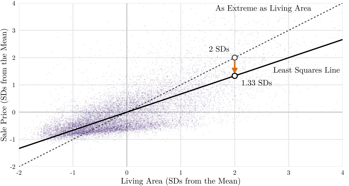
Francis Galton found this pattern in the 1880s: the children of very tall parents were tall, but on average less tall than their parents. He called it regression. The pattern is now called regression toward the mean, and the line that describes it kept the name.
14.3.7 Student’s t-Tests for Individual Coefficients
Using the following formulas, we can always get some estimates from the data, but another sample would give another \(\hat\beta_1\). Is the result convincing?
\[\hat{\beta}_1 = \frac{\sum (X_i - \bar{X})(Y_i - \bar{Y})}{\sum (X_i - \bar{X})^2}, \qquad \hat{\beta}_0 = \bar{Y} - \hat{\beta}_1 \bar{X}\]
Under the assumptions of normal linear regression, this quantity follows a t distribution:
\[\frac{\hat{\beta}_1 - \beta_1}{\operatorname{SE}(\hat\beta_1)} \sim t_{n-k-1}, \ \text{where}\ \operatorname{SE}(\hat\beta_1) = \frac{\hat{\sigma}}{\sqrt{\sum (X_i - \bar{X})^2}}, \quad \hat{\sigma}^2 = \frac{\sum_{i=1}^{n} e_i^2}{n-k-1}\]
- \(\beta_1\): the true slope
- \(\operatorname{SE}(\hat\beta_1)\): the standard error of the slope
- \(\hat\sigma\): the residual standard error, the estimate of the SD of the errors
- \(k\): the number of explanatory variables (\(k = 1\) here; we estimate \(k + 1 = 2\) coefficients, so the t distribution has \(n - 2\) df)
Since \(\sum (X_i - \bar{X})^2 = (n - 1)s_X^2\),
\[\operatorname{SE}(\hat\beta_1) = \frac{\hat\sigma}{s_X\sqrt{n - 1}}\]
The standard error is smaller with a larger \(n\), a larger variance of \(X\) (\(s_X^2\)), and a smaller \(\hat\sigma\). It shrinks with \(\sqrt{n}\), as the standard error of a mean, \(\sigma/\sqrt{n}\), does.
14.3.8 Hypothesis Testing
The usual question is whether \(X\) is related to \(Y\) at all, that is, whether the true slope is 0:
\[H_0 : \beta_1 = 0 \quad H_1 : \beta_1 \neq 0\]
If \(H_0\) is true, the t-value
\[t = \frac{\hat\beta_1}{\operatorname{SE}(\hat\beta_1)}\]
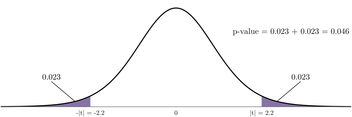
follows the t distribution with \(n - k - 1\) df. The p-value is the probability of a t-value at least as extreme as the observed one if \(H_0\) is true (the shaded area in Figure 14.8). If \(p < 0.05\), the slope is statistically significant at the 0.05 level. As in every test, we may make a Type I or a Type II error.
- Type I error: \(X\) and \(Y\) are not related, but the test says they are.
- Type II error: \(X\) and \(Y\) are related, but the test says they are not.
14.3.9 Confidence Interval of True Parameter \(\beta\)
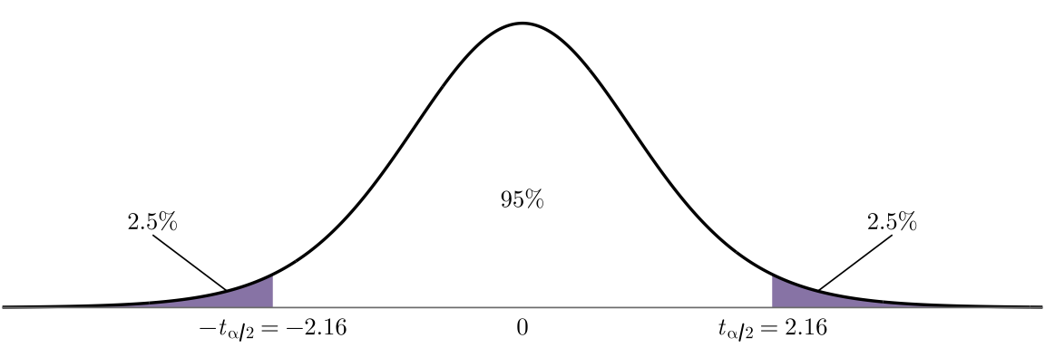
A test asks only whether the slope is 0. A confidence interval gives the range of slopes.4 With probability \(1 - \alpha\), the t statistic lies between \(-t_{\alpha/2}\) and \(t_{\alpha/2}\). Solving for \(\beta_1\) gives the \(1 - \alpha\) confidence interval:
4 R and SPSS report the interval (in R, confint()).
\[\text{estimate} \pm \text{multiplier} \times \operatorname{SE} = \hat{\beta}_1 \pm t_{\alpha/2}\operatorname{SE}(\hat\beta_1)\]
The multiplier \(t_{\alpha/2}\) is the cut-off of the t distribution with \(n - k - 1\) df. The 95% interval excludes 0 exactly when the two-sided test rejects \(H_0\) at the 0.05 level.
14.3.10 Predicting a New Observation
For a new observation with \(X = x_0\), the line predicts \(\hat{Y}_0 = \hat\beta_0 + \hat\beta_1 x_0\). One observation also has its own error \(\varepsilon\), whose standard deviation \(\sigma\) is estimated by the residual standard error \(\hat\sigma = \sqrt{\sum e_i^2 / (n - k - 1)}\), the typical size of a residual.
The prediction stays uncertain by about \(\hat\sigma\). The prediction interval is the range that should contain the \(Y\) of the new observation.5 With a large \(n\), the 95% prediction interval is about
5 In R, predict(m, newdata, interval = "prediction").
\[\hat{Y}_0 \pm 1.96\,\hat\sigma\]
Example 14.7 For a house of \(2,000\) square feet, the linear regression predicts \(\$1,117,054\). With \(\hat\sigma = \$625{,}027\), the 95% prediction interval is from \(-\$0.11\) million to \(\$2.34\) million.
14.3.11 How Much Does the Model Explain the Data?
Sale prices differ from house to house because of location, living area, view, timing, and luck. The variance measures how much they differ, and a model explains a part of it. The total variation of \(Y\) can be split into the part the linear model explains and the residual part, similar to what we did in ANOVA:
\[\underbrace{\sum_{i=1}^{n}(Y_i - \bar{Y})^2}_{\text{total, SST}} = \underbrace{\sum_{i=1}^{n}(\hat{Y}_i - \bar{Y})^2}_{\text{explained, SSM}} + \underbrace{\sum_{i=1}^{n}(Y_i - \hat{Y}_i)^2}_{\text{residual, SSR}}\]
- SST, the total sum of squares: the squared errors of guessing \(\bar{Y}\) for every observation
- SSM, the explained (model) sum of squares: the part explained by the model
- SSR, the residual sum of squares: the part that the model cannot explain
\(R^2\), the coefficient of determination, is the share of the total variation that the model explains:
\[R^2 = \frac{\text{SSM}}{\text{SST}} = 1 - \frac{\text{SSR}}{\text{SST}}\]
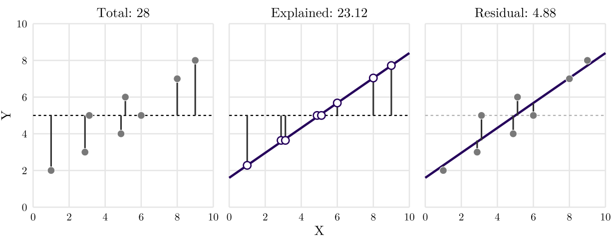
Example 14.8 Rowe et al. (2014) modeled the number of parked cars per occupied unit at 208 King County apartment and condominium properties. Transit access alone (logged) gave \(R^2 = 0.555\). The final model, with seven explanatory variables, has \(R^2 = 0.810\).
What \(R^2\) does not say:
- Whether the model is right. The four data sets of Anscombe’s quartet have the same line and the same \(R^2 = 0.67\).
- Whether the slope matters. Individual observations, such as households, parcels, and sales, depend on much that no data set records. A low \(R^2\) with a clear slope is common for them.
- Which of two models of different outcomes is better. \(R^2\) compares models of the same \(Y\). Different \(Y\) cannot be compared, even price and log price.
14.3.12 Results from R and Interpretations
These are linear regression results from R.
summary(lm(sale_price ~ sqft, data = sales))
Call:
lm(formula = sale_price ~ sqft, data = sales)

Residuals:
     Min       1Q   Median       3Q      Max
-2680199  -305358   -31326   219716 21858935

Coefficients:
              Estimate Std. Error t value Pr(>|t|)
(Intercept) -87731.247  12395.210  -7.078 1.52e-12 ***
sqft           602.393      5.315 113.328  < 2e-16 ***
---
Signif. codes:  0 '***' 0.001 '**' 0.01 '*' 0.05 '.' 0.1 ' ' 1

Residual standard error: 625000 on 16111 degrees of freedom
Multiple R-squared:  0.4436,    Adjusted R-squared:  0.4435
F-statistic: 1.284e+04 on 1 and 16111 DF, p-value: < 2.2e-16- Y, response variable, and X, explanatory variable:
sale_price ~ sqft - Distribution of residuals:
Residuals:, \(e_i = Y_i - \hat{Y}_i\)- The median residual is $31,326 below 0 and the largest is $21.9M above it: a long right tail.
- Estimated coefficients:
Estimate, \(\hat\beta_0\) and \(\hat\beta_1\)- Interpretation: sales that differ by 1 sqft living area differ by $602 in price, on average.
- In social science, the sign of \(\hat\beta\) often matters more than its exact size.
- Standard error of \(\hat\beta\):
Std. Error- Gives the confidence interval:
confint()returns $592 to $613 per square foot.
- Gives the confidence interval:
- t-values and p-values:
t value,Pr(>|t|)- Interpretation: the t-value is 113.33. A t-value this extreme has a probability below \(2 \times 10^{-16}\) (
<2e-16) if the true coefficient is 0.
- Interpretation: the t-value is 113.33. A t-value this extreme has a probability below \(2 \times 10^{-16}\) (
- Residual standard error: \(\hat\sigma = \sqrt{\text{SSR}/(n - k - 1)}\), the typical size of a residual, with \(n - k - 1 = 16{,}111\) df
- Interpretation: a typical prediction misses the sale price by about $625,000.
- R-squared:
Multiple R-squared, \(R^2 = 1 - \text{SSR}/\text{SST}\)- Interpretation: living area explains 44.36% of the variance of sale price.
- Adjusted R-squared:
Adjusted R-squared- Penalizes the number of \(X\)s (prefer models with fewer \(X\)). More helpful than \(R^2\) in comparing models with different numbers of variables.
- F-statistic:
F-statistic- Tests whether all the slopes are 0 at once. With one \(X\), it is the square of the t-value: \(113.33^2 \approx 12{,}840\).
SPSS prints the same numbers in several tables; the lab sessions will discuss more.