10 Estimates and Confidence Intervals
It is better to be vaguely right than exactly wrong.
Carveth Read
10.1 Parametric, Semi-Parametric and Nonparametric
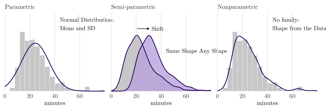
Every distribution we introduced is a family with a few parameters. For example, knowing \(\mu\) and \(\sigma\), we can know the full picture of a normal distribution. Statistical methods differ in the extent to which they rely on assumptions about the underlying distribution family.
- A parametric method assumes the data comes from a fully specified probability distribution family. We will estimate a fixed number of parameters based on the data. This class mostly uses parametric methods; the permutation and rank tests of ch. 11 and 12 are nonparametric.
- A nonparametric method uses data to make inference with as few assumptions as possible (such as no distribution family).
- A semi-parametric method is in between: part of the model has parameters and the rest is learned from data.
10.2 Estimates and Estimators
The parameter (also called the estimand in the context of estimation) is the quantity we want to know, and is fixed (under a Frequentist view). The estimator is the rule that turns sample data into a number, such as \(\hat{p} = x / n\). The estimator is known. The estimate is the calculated estimator for one sample.
A single number reported as the estimate is a point estimate. For example, the usual estimator of population mean \(\mu\) is the sample mean \(\bar{y}\).
Example 10.1 A sample of five monthly rents: $1,200, $1,400, $1,500, $1,600, $3,300. Three example estimators of the population mean \(\mu\):
- the sample mean, \(\bar{y} = \sum y_i / n\): $1,800;
- the sample median: $1,500;
- the first observation, \(Y_1\): $1,200.
But they do not equally estimate the population mean.
10.2.1 Maximum Likelihood
Maximum likelihood is the most important and common-used method to estimate parameters. The idea is we should pick the parameter values under which the observed data is most probable. The likelihood is the probability, or density, of the data sample, read as a function of the parameters. For example, \(n\) independent draws from \(N(\mu, \sigma^2)\), the likelihood of one data point \(y_i\) is the normal PDF at \(y_i\):
\[f(y_i \mid \mu, \sigma^2) = \frac{1}{\sqrt{2\pi\sigma^2}} \exp\Big(-\frac{(y_i - \mu)^2}{2\sigma^2}\Big)\]
The draws are independent, so the joint probability of the sample is the product:
\[L(\mu, \sigma^2) = \prod_{i=1}^n f(y_i \mid \mu, \sigma^2)\]
The maximum likelihood estimator (MLE) is the value of \((\mu, \sigma^2)\) that maximizes \(L\). The log is increasing, so maximizing \(\log L\) gives the same answer, and it turns the product into a sum that is easier to differentiate:
\[\ell(\mu, \sigma^2) = \sum_{i=1}^n \log f(y_i \mid \mu, \sigma^2) = -\frac{n}{2}\log(2\pi\sigma^2) - \frac{1}{2\sigma^2}\sum_{i=1}^n (y_i - \mu)^2\]
The mean. \(\mu\) is only in \(\sum (y_i - \mu)^2\), so \(\ell\) is largest where that sum is smallest. Setting its derivative, \(-2\sum (y_i - \mu)\), to zero gives \(\hat\mu = \bar{y}\).
The variance. With \(\mu = \bar{y}\), set the derivative with respect to \(\sigma^2\) to zero:
\[-\frac{n}{2\sigma^2} + \frac{1}{2\sigma^4}\sum_{i=1}^n (y_i - \bar{y})^2 = 0 \quad\Longrightarrow\quad \hat\sigma^2 = \frac{1}{n}\sum_{i=1}^n (y_i - \bar{y})^2\]
The MLE of \(\mu\) is the sample mean. The MLE of \(\sigma^2\) divides by \(n\). You must remember that the sample variance should divide by \(n - 1\). So that the MLE of \(\sigma^2\) is an biased estimator.
10.3 What Makes a Good Estimator
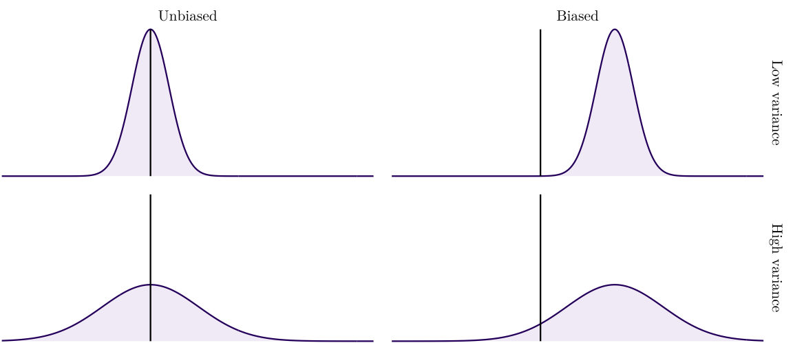
An estimate can be far away the parameter in two ways:
- Sampling error: describes how much an estimate will tend to vary from one sample to the next. It shrinks as \(n\) grows. It is the spread (variance) of the sampling distribution; the square root of the variance is the standard error (SE).
- Bias, or systematic error: a systematic tendency to over- or under-estimate the true population parameters. It pushes every sample the same way and does not shrink as \(n\) grows.
A good estimator keeps both small:
- Unbiased: its sampling distribution centers on the population parameter.
- Efficient: among unbiased estimators, it has the smallest variance, and so the smallest standard error.
- Consistent: it closes in on the parameter as \(n\) grows. For the case of sample mean, this is the law of large numbers.
10.3.1 Reliability and Validity
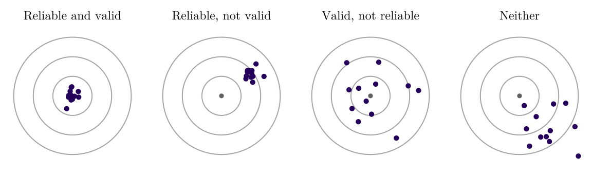
In social science, two parallel concepts are reliability and validity (please read more from Chapter 6 Validity and Reliability: Basic Quantitative Research Methods for Urban Planners. 2020.)
- Reliability: repeating the measurement gives nearly the same result (low variance).
- Validity: the measurement measures what it is meant to measure (low bias).
10.3.2 Bias in Sampling
We design different sample approaches (e.g., simple random sample) to reduce the bias in sampling process. But bias still exists in other ways, for example:
- Selection bias: the procedure systematically favors some units.
- Undercoverage: the frame misses part of the population. For example, an address-based survey misses people without a fixed address.
- Nonresponse bias: those who answer differ from those who do not.
- Response bias: the question’s wording, or the wish to give an acceptable answer, changes what people report.
Example 10.2 The Downtown Seattle Association reports unique downtown visitors to the person: “102% of the number of unique downtown visitors in 2019” State of Downtown 2026. Every number is sourced from Placer.ai, which collects the locations of phones running its partner apps (about 7% of the U.S. population), and scales those phones’ visits up to totals.
- No sampling frame. The phones are whichever ones run the partner apps, not a random draw from the people who come downtown.
- Unknown inclusion probabilities. Placer says each app has its own systematic bias and corrects the data with a model. But these weights cannot be checked.
- Changing phones and methods. Placer revises its algorithm up to once a year, and the revisions change previously reported numbers; new devices also join with their history.
Data with no sampling design have no margin of error. We cannot use these counts to say how close 15.3 million is to the true number of visitors, or whether downtown really had more visitors in 2025 than in 2019.
10.3.3 Mean Squared Error
In order to quantitatively evaluate whether an estimator is good, we can start from its deviation in one sample, \(\hat\theta - \theta\). Then, make the average of square deviation. We call this quantity mean squared error (MSE): the average squared deviation over all possible samples:
\[\operatorname{MSE}(\hat\theta) = E\big[(\hat\theta - \theta)^2\big]\]
MSE is one of the most important indicator to evaluate the performance of an estimator. We can decompose MSE into two parts: bias and variance, which reveals one fundamental concept in machine learning called bias-variance trade off. If you are interested, check this Machine Learning Fundamentals: Bias and Variance video with Josh Starmer.
\[\operatorname{MSE}(\hat\theta) = \underbrace{\big(E(\hat\theta) - \theta\big)^2}_{\text{bias}^2} + \underbrace{\operatorname{Var}(\hat\theta)}_{\text{variance}}\]
10.4 Confidence Intervals
By the central limit theorem, for a large sample the sample mean is approximately normal, centered on \(\mu\), with SD equal to its standard error. The standard error of a sample mean is \(\sigma / \sqrt{n}\).
A confidence interval reports an estimate as a range:
\[\text{estimate} \pm \text{multiplier} \times \operatorname{SE}\]
The half-width, multiplier \(\times\) SE, is the margin of error (MOE). The multiplier is set by the confidence level \(C\) and by the sampling distribution of the estimate.
When that distribution is normal, as the central limit theorem gives for large samples, the multiplier is \(z^*\), a z-score on the standard normal curve.
| Confidence level \(C\) | Each tail | \(P(Z < z^*)\) | \(z^*\) |
|---|---|---|---|
| 50% | 0.2500 | 0.7500 | 0.674 |
| 80% | 0.1000 | 0.9000 | 1.282 |
| 90% | 0.0500 | 0.9500 | 1.645 |
| 95% | 0.0250 | 0.9750 | 1.960 |
| 99% | 0.0050 | 0.9950 | 2.576 |
| 99.9% | 0.0005 | 0.9995 | 3.291 |
Example 10.3 A survey of 400 renter households finds that 200 are cost-burdened. Each household is a Bernoulli variable: \(Y = 1\) if burdened and 0 if not, with expectation \(E(X) = p\) and SD \(\sigma = \sqrt{p(1 - p)}\). The sample share \(\hat{p}\) is the mean of the \(X\)s, so its SE is \(\sigma / \sqrt{n} = \sqrt{p(1 - p)/n}\), with \(\hat{p}\) in place of the unknown \(p\):
\[\hat{p} = \frac{200}{400} = 0.5, \qquad \sigma \approx \sqrt{0.5 \times 0.5} = 0.5, \qquad \operatorname{SE} = \frac{0.5}{\sqrt{400}} = \frac{0.5}{20} = 0.025\]
Based on the Central limit theorem, \(\hat{p}\) is approximately normally distributed.
- the 95% interval is \(0.5 \pm 1.96 \times 0.025 = 0.5 \pm 0.049\), from 45.1% to 54.9%
- the 90% interval is \(0.5 \pm 1.645 \times 0.025 = 0.5 \pm 0.041\), from 45.9% to 54.1%
10.4.1 What the 95% means
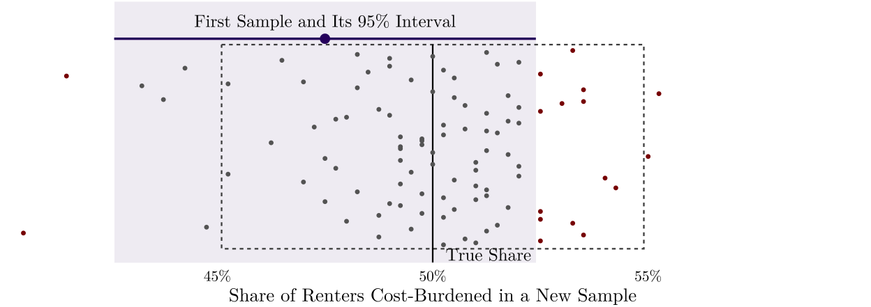
The confidence interval changes from sample to sample.
- Before the sample is drawn, the procedure has a 95% chance of producing an interval that covers the parameter. In the following figure, 95 of 100 intervals cover the true parameter.
- Once a sample is drawn, its confidence interval, 45.1% to 54.9%, is fixed. we can be 95% confident that it captures the true parameter. This confidence comes from the fact that 95% of all intervals generated by this methodology will successfully contain the true parameter.
Check Frequentist Inference on Seeing Theory.

A 95% confidence interval is NOT:
- A probability for this interval. “The true parameter is between 45.1% and 54.9% with probability 95%” treats the parameter as random, which is incorrect under Frequentist view. However, a Bayesian view treats unknown parameters as random variables and they have a term credible interval.
- A prediction interval for future estimates. A common misconception is that a 95% confidence interval dictates a 95% probability of capturing the point estimate of a future sample. In reality, only 83.4% second sample’s estimate will fall inside the original confidence interval, because both the baseline interval and the new estimate are subject to separate random variation.
- Protection against bias. The confidence interval only quantifies sampling error. A biased sample will give a biased interval.
Example 10.4 Seattle’s 2020 Urban Forest Management Plan reports 28% canopy cover from a 2016 LiDAR assessment, “with a +/- 1% margin of error” (quote below), and says that earlier assessments used other methods and cannot be compared with it. What is the meaning of “+/- 1% margin of error” in this context?
A formal accuracy assessment was not performed for the study, but similar studies have shows to have a margin of error of +/- 1%.
10.4.2 Comparing with a Threshold
If the error margin completely clears the threshold, the data gives a clear answer (at least at current confidence level). If the error margin overlaps with the threshold, the result is inconclusive.
Example 10.5 New York City tries to keep rent stabilization only while its rental vacancy rate is at most 5% (Emergency Tenant Protection Act). The Housing and Vacancy Survey put the 2021 rate at 4.54%, with a 90% interval of 4.10% to 4.98% (reported by the report). In the report, they describe that “MOEs were calculated by multiplying the standard error of the estimate by 1.645.” Therefore:
\[\operatorname{SE} = \frac{0.44\%}{1.645} = 0.27\%, \qquad 95\% \text{ interval: } 4.54\% \pm 1.96 \times 0.27\% = 4.02\% \text{ to } 5.06\%\]
The 90% interval lies below 5% but the 95% interval contains it, so whether 2021 vacancy was below the line depends on a confidence level that the law does not specify.
10.5 Margins of Error in the ACS
The Census Bureau publishes every ACS estimate with a margin of error at the 90% level:1
1 The Bureau computes these standard errors from 80 sets of replicate weights, not from the simple-random-sample formulas of this chapter, because the ACS is not a simple random sample.
\[\operatorname{MOE} = 1.645 \times \operatorname{SE}, \qquad \operatorname{SE} = \frac{\operatorname{MOE}}{1.645}\]
So the 90% confidence interval is the \(\text{estimate} \pm \text{MOE}\). The MOE is not a sign of bad data. Nor is it the whole uncertainty: it measures the variance of the estimate, not its bias.
10.5.1 Coefficient of Variation
The coefficient of variation (CV) measures the SE relative to the estimate (a way to say precision):
\[\operatorname{CV} = \frac{\operatorname{SE}}{\text{estimate}}\]
For example, Census Tract 4001, Alameda County, California has \(\operatorname{CV} = 244 / 3{,}035 = 8.1\%\).
There is no official threshold for a precise enough estimate. A common convention, used by Esri:
- \(CV < 12\%\) high precision
- \(12\% - 40\%\) medium precision (use with caution)
- \(CV > 40\%\) low precision
Example 10.7 Jurjevich et al. (2018) interviewed 7 planners and surveyed 200 planners. They found that many planners do not understand the uncertainty in ACS estimates, find it difficult to explain to stakeholders, and leave MOEs out of their reports altogether. They recommend five practices:
- Report MOEs.
- Say so when MOEs are not reported.
- Give context for how precise the estimates are, for example with the CV.
- Consider ways to reduce the uncertainty, such as combining areas or years.
- Before saying that two ACS estimates differ, check the difference against its own margin of error.
10.5.2 Combining Estimates
A derived estimate is one we build ourselves from published estimates, such as a study area added up from several tracts. It comes with no MOE, but the Census Bureau’s ACS handbook gives approximate formulas.2 For a sum:
2 In R, the tidycensus functions moe_sum(), moe_prop(), moe_ratio(), and moe_product() implement these formulas.
\[\operatorname{MOE}(\hat{X}_1 + \hat{X}_2 + \cdots + \hat{X}_n) = \pm\sqrt{[\operatorname{MOE}(\hat{X}_1)]^2 + [\operatorname{MOE}(\hat{X}_2)]^2 + \cdots + [\operatorname{MOE}(\hat{X}_n)]^2}\]
The formulas are approximations: they treat the estimates as independent, and the more estimates are combined, the further the approximate MOE can drift from the MOE the Census Bureau would compute from the full survey data.
Example 10.8 Combine Census Tracts 4001 and 4002 of Table 3.8. The estimate is \(3{,}035 + 1{,}983 = 5{,}018\), and the MOE is
\[\sqrt{402^2 + 209^2} \approx 453\]
The combined CV is \((453 / 1.645) / 5{,}018 = 5.5\%\), lower than the CV of either tract (8.1% and 6.4%). Aggregating trades geographic detail for higher precision.
The Chapter 8 in ACS handbook also gives formulas for derived estimates other than sums, such as ratios, proportions, and products.
| Derived estimate | Approximate MOE |
|---|---|
| Sum or difference, \(\hat{X}_1 \pm \cdots \pm \hat{X}_n\) | \(\pm\sqrt{[\operatorname{MOE}(\hat{X}_1)]^2 + \cdots + [\operatorname{MOE}(\hat{X}_n)]^2}\) |
| Proportion, \(\hat{P} = \hat{X} / \hat{Y}\), \(X\) a subset of \(Y\) | \(\frac{1}{\hat{Y}} \sqrt{[\operatorname{MOE}(\hat{X})]^2 - \hat{P}^2 [\operatorname{MOE}(\hat{Y})]^2}\) |
| Percentage, \(\hat{Q} = 100\% \times \hat{P}\) | \(100\% \times \operatorname{MOE}(\hat{P})\) |
| Ratio, \(\hat{R} = \hat{X} / \hat{Y}\), \(X\) not a subset of \(Y\) | \(\frac{1}{\hat{Y}} \sqrt{[\operatorname{MOE}(\hat{X})]^2 + \hat{R}^2 [\operatorname{MOE}(\hat{Y})]^2}\) |
| Percent change, \(100 \times (\hat{X} - \hat{Y}) / \hat{Y}\) | \(100 \times \operatorname{MOE}(\hat{X} / \hat{Y})\), by the ratio formula |
| Product, \(\hat{X} \times \hat{Y}\) | \(\sqrt{\hat{X}^2 [\operatorname{MOE}(\hat{Y})]^2 + \hat{Y}^2 [\operatorname{MOE}(\hat{X})]^2}\) |
10.6 Unknown SD and the t Distribution
So far the population SD \(\sigma\) has been treated as known, so that the SD of a sample mean is \(\sigma / \sqrt{n}\). However, we do not know the population SD \(\sigma\) in most cases.
For a numerical variable, such as a rent or a commute time, \(\sigma\) is a second unknown, separate from the mean \(\mu\), and is estimated by the sample SD \(s\). Because \(s\) is measured around \(\bar{y}\) rather than \(\mu\), it has \(n - 1\) degrees of freedom (df). Since \(s\) itself varies from sample to sample (adds uncertainity to the estimates of \(\mu\)), \(z^*\) is replaced by a larger multiplier \(t^*\) from the t distribution with \(n - 1\) df:
\[\bar{y} \pm t^*_{n-1} \times \frac{s}{\sqrt{n}}\]
The t distribution has the bell shape of the normal curve with heavier tails, and it approaches the normal as the degrees of freedom grow.
| df | 90% | 95% | 99% |
|---|---|---|---|
| 1 | 6.314 | 12.706 | 63.657 |
| 2 | 2.920 | 4.303 | 9.925 |
| 3 | 2.353 | 3.182 | 5.841 |
| 4 | 2.132 | 2.776 | 4.604 |
| 5 | 2.015 | 2.571 | 4.032 |
| 10 | 1.812 | 2.228 | 3.169 |
| 20 | 1.725 | 2.086 | 2.845 |
| 30 | 1.697 | 2.042 | 2.750 |
| 50 | 1.676 | 2.009 | 2.678 |
| 100 | 1.660 | 1.984 | 2.626 |
Example 10.9 Five commute time: 12, 18, 24, 31 and 40 minutes and how to estimate 95% CI? We can first estimate both sample mean and sample SD: \(\bar{y} = 25\), \(s = 10.95\).
SE of sample mean is \(\operatorname{SE} = 10.95/\sqrt{5} = 4.90\). With \(n - 1 = 4\) df, \(t^* = 2.776\) (Table 10.3)3:
3 The multiplier \(t^*\) can be found via t-distribution table, or using qt(0.975, df = 4) in R (using 0.975 because qt(p, df) shows the value with probability p below it.)
\[25 \pm 2.776 \times 4.90 = 25 \pm 13.6, \text{ from 11.4 to 38.6 minutes}\]
If we don’t use t distribution, \(z^* = 1.96\) the interval would be \(25 \pm 9.6\), from 15.4 to 34.6: narrower, and too narrow for a sample of five.
With \(z^*\), the intervals are too narrow: at \(n = 5\), about 12% of them miss the mean.
The t interval still assumes roughly normal data, or a sample large enough for the central limit theorem. For a small sample with a few extreme values using the bootstrap (optional) would be better.
10.6.1 Why n - 1?
As in lecture 2 (Figure 2.5, Figure 2.6), we briefly mention why we need to divide by \(n-1\). Another explanation (tricky one) is using idea of Degree of Freedom (df). To put it informally, think of each independent data point as a unit of currency deposited into a statistical bank account. Every time you estimate a new parameter in your analysis, you ‘spend’ one unit of that currency. The remaining balance left over in your account is your budget of flexibility and we call your degrees of freedom. In the case of sample SD, it is built from \(\bar y\) and we spent one ‘degree of freedom’.
\[s = \sqrt{\frac{1}{n - 1}\sum_{i=1}^{n} (y_i - \bar{y})^2}\]
Another visual way can be the sample SD is built from the deviations \(y_i - \bar{y}\) and we know that the deviations always add to 0. Once \(n - 1\) of them are known, the last one is fixed, so only \(n - 1\) deviations are free to vary.
10.6.2 Where the t Distribution Comes From
The multiplier \(z^*\) came from the distribution of the standardized mean. Replacing \(\sigma\) by \(s\) changes that distribution:
\[\frac{\bar{y} - \mu}{\sigma / \sqrt{n}} \sim N(0, 1) \qquad \longrightarrow \qquad \frac{\bar{y} - \mu}{s / \sqrt{n}} \sim t_{n-1}\]
The only difference is the denominator. With \(\sigma\) it is fixed; with \(s\) it varies from sample to sample, a second source of variation. A sample with a small \(s\) gives a large value, so the t distribution with \(n - 1\) df has heavier tails than the normal, and its 95% multiplier \(t^*\) is larger than 1.96.
Start from a normal sample. Two facts:
- If \(\sigma\) were known, \(Z = (\bar{y} - \mu) / (\sigma / \sqrt{n})\) would be standard normal based on central limit theorem.
- \(s^2\) varies from sample to sample: \((n - 1)s^2/\sigma^2\) follows a chi-square distribution with \(n - 1\) degree of freedom, and for normal data it is independent of \(\bar{y}\).
Replacing \(\sigma\) by \(s\) divides \(Z\) by \(s/\sigma\), a random amount:
\[T = \frac{\bar{y} - \mu}{s / \sqrt{n}} = \frac{\dfrac{\bar{y} - \mu}{\sigma / \sqrt{n}}}{\dfrac{s}{\sigma}} = \frac{Z}{s / \sigma} = \frac{Z}{\sqrt{\chi^2_{n-1} / (n - 1)}}\]
A standard normal divided by the square root of an independent chi-square over its df has the t distribution with that many df. The \(\sigma\) in the numerator and the one in the denominator cancel. The value of \(T\) still involves the unknown \(\mu\), but its distribution does not depend on \(\mu\) or \(\sigma\), so \(t^*\) can be found without knowing either. Then
\[P\left(-t^* \le \frac{\bar{y} - \mu}{s / \sqrt{n}} \le t^*\right) = 0.95 \quad\Longrightarrow\quad P\left(\bar{y} - t^* \frac{s}{\sqrt{n}} \le \mu \le \bar{y} + t^* \frac{s}{\sqrt{n}}\right) = 0.95\]
which is the interval \(\bar{y} \pm t^* s / \sqrt{n}\).
10.7 Choosing the Sample Size
Example 10.10 A city wants to estimate the share of renters who are cost-burdened; and wants to have interval within \(\pm 5\) percentage points at 95% confidence (MOE of 0.05).
The MOE of a share is \(z^* \times \operatorname{SE}\), so set it equal to the target:
\[1.96\times\sqrt{\frac{p(1-p)}{n}} = 0.05\]
Then we solve for \(n\):
\[\frac{p(1-p)}{n} = \left(\frac{0.05}{1.96}\right)^2 \quad\Longrightarrow\quad n = p(1-p) \times \left(\frac{1.96}{0.05}\right)^2 = p(1-p) \times 1{,}536.64\]
The share is unknown before the survey. \(p(1-p)\) is largest at \(p = 0.5\), where it is 0.25, so 0.25 gives a sample large enough whatever the share turns out to be:
\[n = 0.25 \times 1{,}536.64 = 384.16\]
Round up to 385 responses and it is the sample size.
10.8 The Bootstrap
Many planning statistics have no simple SE formula. The bootstrap estimates the sampling distribution from the sample itself (Efron and Hastie 2016):
- Draw \(n\) cases from the sample with replacement, so that some cases appear more than once and some not at all. This is a bootstrap sample.
- Compute the statistic on the bootstrap sample.
- Repeat thousands of times.
- The middle 95% of the bootstrap statistics is an approximate 95% confidence interval, the percentile interval.
However, the bootstrap will inherit every bias in how the sample was drawn.
Check Frequentist Inference on Seeing Theory.
Example 10.11 A sample of 40 rents (simulated) has a median of $1,600. In 5,000 bootstrap samples the median ranges widely, and its middle 95% runs from $1,485 to $1,930. The interval is not symmetric around $1,600, which no formula of the form estimate \(\pm\) MOE could show.

10.9 Summary: Which Interval
For estimating a population mean, the interval depends on the sample size, on the shape of the population, and on whether \(\sigma\) is known.
