With four parameters I can fit an elephant, and with five I can make him wiggle his trunk.
John von Neumann
15.1 Adding Explanatory Variables
In simple regression, \(\hat\beta_1\) also includes the effects of other variables that are correlated with \(X\). For example, newer houses are larger, so the slope of year built alone partly reflects living area. Adding those variables to the model controls for them. With \(k\) explanatory variables, the model is
OLS still minimizes the sum of squared residuals, and each \(\hat\beta_j\) has its own standard error, t-test, and confidence interval, with \(n - k - 1\) df. The R output is read as before:
summary(lm(sale_price ~ sqft + year_built, data = sales))
Call:
lm(formula = sale_price ~ sqft + year_built, data = sales)

Residuals:
     Min       1Q   Median       3Q      Max
-2801751  -295449   -35632   223181 21842508

Coefficients:
              Estimate Std. Error t value Pr(>|t|)
(Intercept)  6.636e+06  3.079e+05   21.55   <2e-16 ***
sqft         6.354e+02  5.452e+00  116.55   <2e-16 ***
year_built  -3.440e+03  1.574e+02  -21.86   <2e-16 ***
---
Signif. codes:  0 '***' 0.001 '**' 0.01 '*' 0.05 '.' 0.1 ' ' 1

Residual standard error: 616000 on 16110 degrees of freedom
Multiple R-squared:  0.4596,    Adjusted R-squared:  0.4595
F-statistic:  6850 on 2 and 16110 DF,  p-value: < 2.2e-16
\(\beta_j\) is the expected change in \(Y\) for a one-unit increase in \(X_j\), holding all other explanatory variables constant:
sqft: the expected change in price for 1 sqft increase in area, holding year built constant, is $635 (95% CI: $625 to $646).
With living area alone, the slope was $602.
year_built: the expected change in price for a house built 1 year later, holding living area constant, is \(-\$3{,}440\).
Residual standard error and R-squared: \(\hat\sigma = \$616{,}000\) with \(n - k - 1 = 16{,}113 - 2 - 1 = 16{,}110\) df, and \(R^2 = 0.4596\).
With living area alone, \(\hat\sigma = \$625{,}000\) and \(R^2 = 0.4436\).
15.2 What to Control For
15.2.1 Omitted Variable Bias
If a variable \(X_2\) that affects \(Y\) is omitted, the coefficients of the included variables that are correlated with \(X_2\) are biased (omitted variable bias). In a sample, the slope of \(Y\) on \(X_1\) alone is:
\[\underbrace{\tilde\beta_1}_{X_2 \text{ omitted}} = \underbrace{\hat\beta_1}_{X_2 \text{ held constant}} + \overbrace{\underbrace{\hat\beta_2}_{\text{effect of } X_2 \text{ on } Y}\;\underbrace{\hat\delta_1}_{\text{slope of } X_2 \text{ on } X_1}}^{\text{omitted variable bias}}\]
where \(\hat\beta_1\) and \(\hat\beta_2\) are the slopes from the regression of \(Y\) on both variables, and \(\hat\delta_1\) is the slope from the regression of \(X_2\) on \(X_1\).
The bias is \(\hat\beta_2\,\hat\delta_1\). It is 0 only if \(X_2\) does not affect \(Y\) (\(\hat\beta_2 = 0\)) or is not correlated with \(X_1\) (\(\hat\delta_1 = 0\)).
15.2.2 Confounders, Mediators, and Colliders
In a randomized experiment, a random mechanism assigns the treatment \(X\), so no other variable affects \(X\). In an observational study, any variable that affects both \(X\) and \(Y\) is a confounder, and we need to control for it.
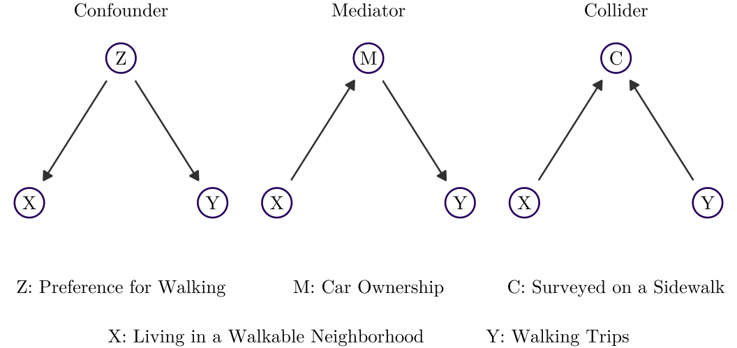
A causal diagram draws one node for each variable and one arrow for each direct effect (Pearl and Mackenzie 2018). Figure 15.1 shows three positions of a third variable:
Pearl, Judea, and Dana Mackenzie. 2018. The Book of Why: The New Science of Cause and Effect. Basic Books.
a confounder\(Z\) affects both \(X\) and \(Y\) – should be controlled
a mediator\(M\) lies on the path from \(X\) to \(Y\) – should not
a collider\(C\) is affected by both \(X\) and \(Y\) – should not
Figure 15.1: Three positions of a third variable.
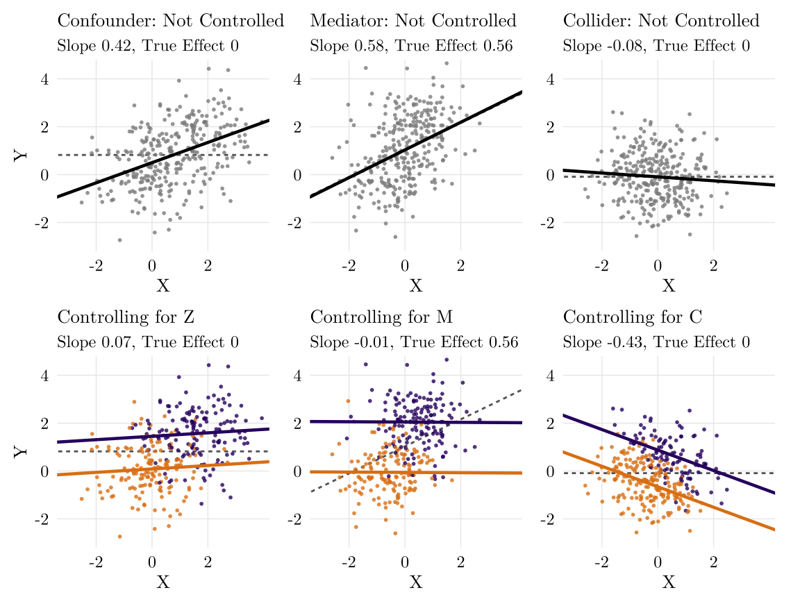
Figure 15.2: X and Y with a third variable that is 0 or 1. Top: the least squares line of Y on X. Bottom: Y on X and the third variable, one line per group (orange 0, purple 1) with a common slope.
In figure above, the dashed line is the true effect of \(X\) on \(Y\).
Confounder: \(X\) has no effect on \(Y\); \(Z\) raises both. Controlling for \(Z\) moves the slope of \(X\) from 0.42 to 0.07, close to the true effect, 0.
Mediator: \(X\) raises \(M\), and \(M\) raises \(Y\), so the true effect of \(X\), 0.56, runs entirely through \(M\). Controlling for \(M\) moves the slope from 0.58 to \(-0.01\).
Collider: \(X\) and \(Y\) are unrelated, and \(C = 1\) when \(X + Y\) is large. Controlling for \(C\) moves the slope from \(-0.08\) to \(-0.43\), though the true effect is 0.
15.3 Beyond a Straight Line
A linear regression is linear in the \(\beta\)s, not necessarily in \(X\). So that we can use make them beyond a straight line.
15.3.1 Log Transformation
Right-skewed variables, such as prices, incomes, and permit times, are often logged. With a logged variable, the coefficient is interpreted in percent:
Model
Interpretation of \(\hat\beta_1\)
Example: \(\hat\beta_1 = 0.5\)
\(Y = \beta_0 + \beta_1 X\)
One-unit increase in \(X\): \(Y\) changes by \(\hat\beta_1\) units
\(X\) one unit higher: \(Y\) 0.5 units higher
\(\log Y = \beta_0 + \beta_1 X\)
One-unit increase in \(X\): \(Y\) changes by \(100(e^{\hat\beta_1} - 1)\%\), about \(100\hat\beta_1\%\) when \(\hat\beta_1\) is small
\(X\) one unit higher: \(Y\) 65% higher (\(e^{0.5} = 1.65\)), not 50%
\(Y = \beta_0 + \beta_1 \log X\)
1% increase in \(X\): \(Y\) changes by about \(\hat\beta_1 / 100\)
\(X\) 1% higher: \(Y\) 0.005 units higher
Table 15.1: Interpretation of \(\hat\beta_1\) when \(Y\) or \(X\) are logged (natural logs).
15.3.2 Categorical Explanatory Variables
A categorical variable enters the model as dummy variables: one 0/1 variable for each category except one (baseline). The omitted category is the reference group, and the coefficient of each dummy is the difference in the mean of \(Y\) between its category and the reference group, holding the other variables constant.1 Changing the reference group changes the coefficients, but not the fitted values or \(R^2\). With a numerical \(X\) and one dummy \(D\),
1 R creates the dummies from a character or factor variable and takes the first category in alphabetical order as the reference group; relevel() changes it.
\[Y = \beta_0 + \beta_1 X + \beta_2 D + \varepsilon\]
the intercept is \(\beta_0\) when \(D = 0\) and \(\beta_0 + \beta_2\) when \(D = 1\): these two lines are parallel with the same slope \(\beta_1\).
A set of dummy variables for groups is called fixed effects. Each group has its own intercept, so the other coefficients use only the variation within groups, and an omitted variable that is constant within a group cannot bias them.
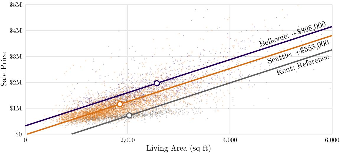
Example 15.1 For the sales in Kent, Seattle, and Bellevue, with Kent as the reference group, lm(sale_price ~ sqft + city) fits
where \(\text{Seattle}_i = 1\) for a sale in Seattle and 0 otherwise, and likewise \(\text{Bellevue}_i\); a sale in Kent has both equal to 0. Each city has its own intercept, and the three share the slope \(\beta_1\):
An interaction term is the product of two explanatory variables. It allows the slope of one variable to depend on the value of the other. For example, with a dummy \(D\),
\[Y = \beta_0 + \beta_1 X + \beta_2 D + \beta_3 X D + \varepsilon\]
the slope of \(X\) is:
\(\beta_1\) when \(D = 0\)
\(\beta_1 + \beta_3\) when \(D = 1\)
With a categorical variable, one interaction term per dummy gives one slope of \(X\) per group.2 Right now, we can have both different intercepts and slopes for each group.
2 In R, lm(y ~ x * group).
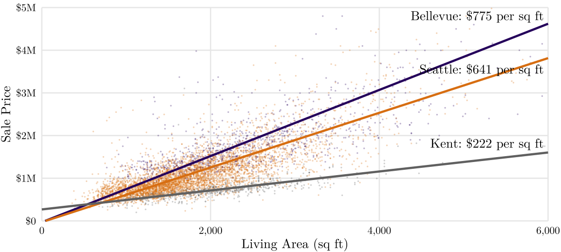
Example 15.2 For the same three cities, lm(sale_price ~ sqft * city) adds two interaction terms:
Seattle’s slope - Kent’s; so Seattle’s \(222.5 + 418.4\)
sqft:cityBellevue
\(\hat\beta_5\)
\(552.7\)
Bellevue’s slope - Kent’s; so Bellevue’s \(222.5 + 552.7\)
With an interaction, the difference between the cities depends on living area, and the coefficients of the city dummies alone compare the cities at 0 sq ft.
Figure 15.4: Living area and sale price in Bellevue, Seattle, and Kent, King County sales of 2025, with one least squares line per city.
15.4 Checking the Assumptions
The assumptions of normal linear regression are mostly about the errors, which are never observed, so we check them on the residuals (as the estimation of errors).
Assumption
Check
Common response
Linearity
Residual plot: the mean of the residuals is not 0 at every \(\hat{Y}\) (a curve)
Log \(X\) or \(Y\), add \(X^2\), use other models
Independence
Residuals by group, in time order, on a map
Cluster-robust standard errors, fixed effects, models for correlated data
Equal variance
Residual plot: the variance of the residuals changes with \(\hat{Y}\) (a fan shape)
Log \(Y\), robust standard errors
Normality
Normal Q-Q plot
With a large \(n\), none (CLT); with a small \(n\), check for outliers
No multicollinearity
Correlation matrix of the \(X\)s; VIF > 5 or 10
Drop or combine the correlated variables
Table 15.2: Checking the assumptions.
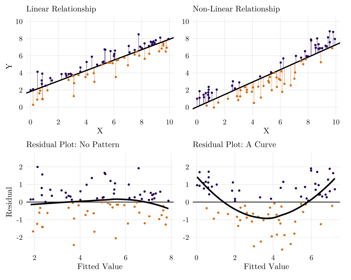
The main tool is the residual plot: the residuals \(e_i\) against the fitted values \(\hat{Y}_i\).3 When the assumptions hold, the residuals have mean 0 and about the same variance at every fitted value, with no pattern.4
3 In R, plot(m, which = 1) draws the residual plot of a model m, and plot(m, which = 2) its normal Q-Q plot. In SPSS: Linear Regression, Plots, *ZRESID against *ZPRED, and Normal probability plot.
4 Each assumption also has a formal test, such as Breusch-Pagan for equal variance, Shapiro-Wilk for normality, Durbin-Watson for autocorrelation over time, and Moran’s \(I\) for spatial autocorrelation.
15.4.1 Linearity
Linearity says that the mean of \(Y\) is a linear function of \(X\), \(E[Y \mid X] = \beta_0 + \beta_1 X\), so the errors have mean 0 at every value of \(X\).
If the relationship is non-linear, the residual plot shows a curve. With several explanatory variables, also plot the residuals against each \(X_j\), because a non-linear relationship with one \(X_j\) may not show against \(\hat{Y}\).
Figure 15.5: Simulated data with a linear (left) and a non-linear (right) relationship. Top: the data and the least squares line, with each residual as a segment. Bottom: the residual plot of the same data, with a smooth curve. Purple: positive residuals. Orange: negative residuals.
If it fails, the coefficients themselves are wrong. Avoid using linear regressions or transform the variables to make the model is still linear in the \(\beta\)s. For example:
Log \(X\) or \(Y\): \(\log Y = \beta_0 + \beta_1 \log X + \varepsilon\)
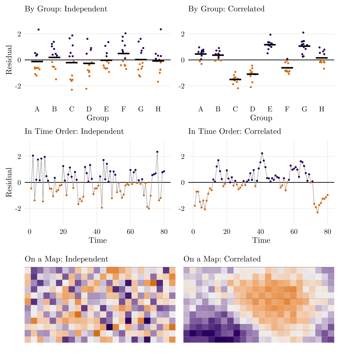
Independence says that the errors of different observations are not correlated: \(\operatorname{Cov}(\varepsilon_i, \varepsilon_j) = 0\) for \(i \neq j\). The residual plot cannot show it. Errors are usually correlated in one of three ways, each with its own plot of the residuals
By group (clustered data): the mean residual of each group differs from 0.
In time order (autocorrelation): residuals close in time have the same sign.
On a map (spatial autocorrelation): the residuals of nearby observations are similar.
Figure 15.6: Simulated residuals, independent (left) and correlated (right). By group: the residuals of each group and their mean (black). In time order: the residuals in the order of the observations. On a map: one rectangle per observation. Purple: positive residuals. Orange: negative residuals.
If it fails, the coefficients (\(\beta\)) are still unbiased, but their standard errors are too small, then CI and p-value are incorrect. So that, we can use:
Cluster-robust standard errors allow \(\operatorname{Cov}(\varepsilon_i, \varepsilon_j) \neq 0\) for two observations in the same group (cluster), such as two sales in one city. The coefficients do not change.5
Fixed effects for the groups.
Models for correlated data, such as multilevel models and spatial regression models.
5 In R, sandwich::vcovCL(), with the groups as clusters.
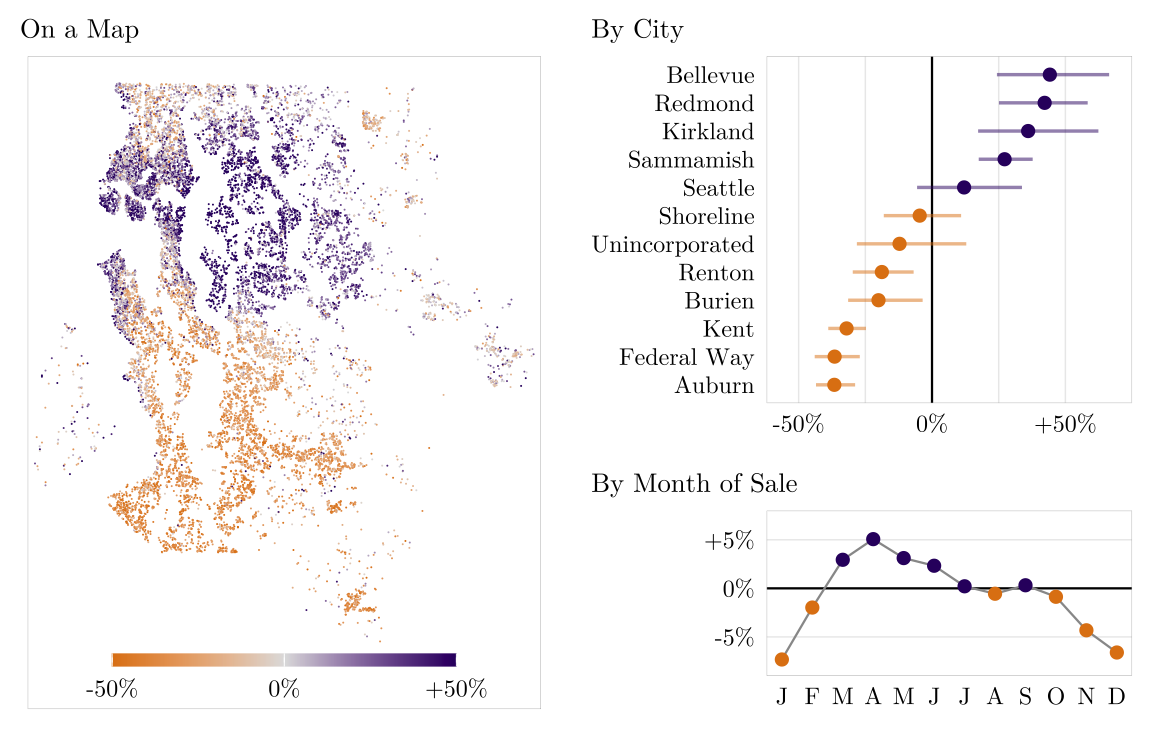
Example 15.3 In the case, the residuals of the regression of log price on log living area are correlated in all three ways:
By city: the median residual is \(+44\%\) in Bellevue and \(-37\%\) in Auburn.
By month of sale: the mean residual is \(-7\%\) in January and \(+5\%\) in April.
On the map: the residuals are positive in Seattle and on the Eastside, and negative in the south.
Figure 15.7: Residuals of log price on log living area, King County sales of 2025, as percentages above or below the predicted price.
In the regression of log price on log living area, \(\hat\beta_1 = 0.85\) with \(\operatorname{SE}(\hat\beta_1) = 0.0069\), and the 95% confidence interval is 0.83 to 0.86.
With the 40 cities as clusters, the cluster-robust standard error of \(\hat\beta_1\) is 0.053, 7.7 times as large, and the 95% confidence interval is 0.74 to 0.95. \(\hat\beta_1\) does not change.
15.4.3 Equal Variance
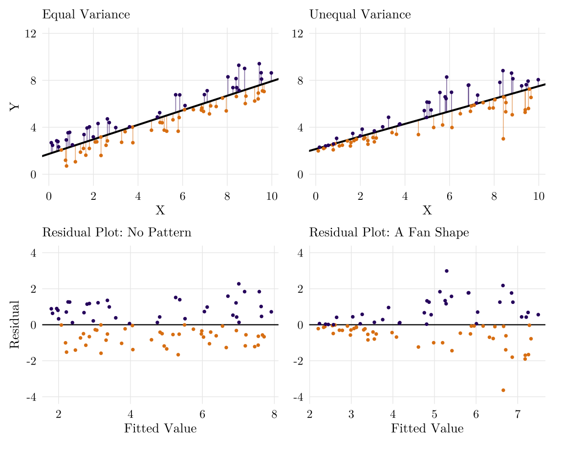
Equal variance (homoscedasticity) says that \(\operatorname{Var}(\varepsilon_i) = \sigma^2\) at every value of \(X\). With unequal variance (heteroscedasticity), the variance of the residuals changes with the fitted value \(\hat{Y}\). Most often it increases, and the residual plot has a fan shape.
This is common for right-skewed variables such as prices and incomes: the errors of expensive houses have a larger variance than the errors of cheap houses.
Figure 15.8: Simulated data with equal variance (left) and with a variance that increases with X (right). Top: the data and the least squares line. Bottom: the residual plot.
If it fails, the coefficients are still unbiased, but their standard errors can be too small or too large:
Log \(Y\): when the SD of \(Y\) is proportional to its mean, \(\log Y\) has about the same variance at every \(X\).
Robust standard errors (heteroscedasticity-consistent standard errors) do not assume a constant \(\sigma^2\). The coefficients do not change.6
6 In R, sandwich::vcovHC().
15.4.4 Normality
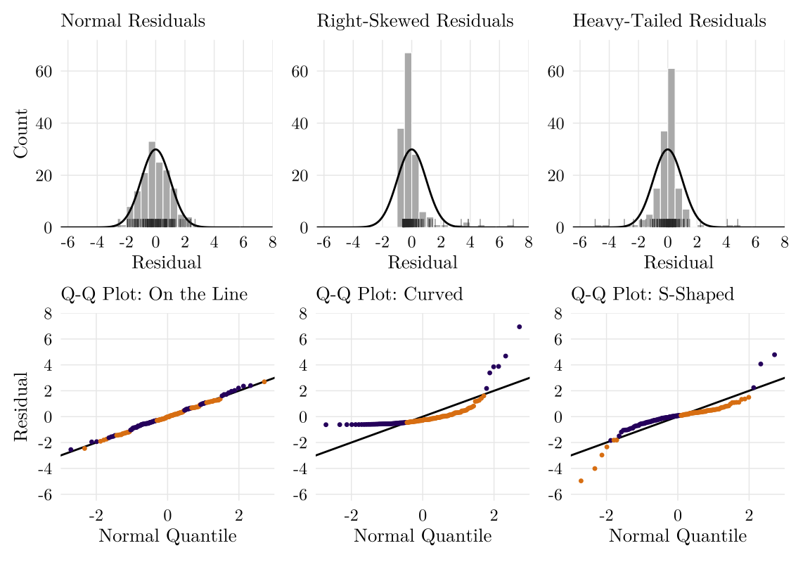
Normality says that \(\varepsilon_i \sim N(0, \sigma^2)\). The normal Q-Q plot plots the quantiles of the residuals against the quantiles of a normal distribution:
If the residuals are normal, the points are on the line.
With right-skewed residuals, the points are above the line at both ends.
With heavy tails, they are below the line at the left end and above it at the right end.
Figure 15.9: A normal, a right-skewed, and a heavy-tailed distribution. Top: histograms of residuas. Bottom: normal Q-Q plots.
If it fails, the coefficients are still unbiased and their standard errors are still correct. Only the t distribution behind the p-values and the multiplier \(t_{\alpha/2}\) is no longer exact:
With a large \(n\), they are still approximately valid, by the central limit theorem (CLT).
With a small \(n\), they are approximate. Check for outliers before transforming \(Y\).
15.4.5 Multicollinearity
Perfect multicollinearity is when one \(X\) is a linear combination of the others, such as \(X_3 = X_1 + X_2\), then the coefficients cannot be estimated.7Multicollinearity is when the explanatory variables are highly, but not perfectly, correlated.
7 In R, lm() reports NA for one of the coefficients.
The coefficients are still unbiased and the predicted values \(\hat{Y}\) are not affected, but the standard errors of the correlated variables are large, so their t-tests are often not significant:
where \(R_j^2\) is the \(R^2\) of the regression of \(X_j\) on the other explanatory variables, and \(\text{VIF}_j\) is the variance inflation factor.
Figure 15.10: Simulated data with two explanatory variables correlated at \(r\) and the estimates \(\hat\beta_1\) and \(\hat\beta_2\) with their 95% CIs.
To check, use a correlation matrix of the explanatory variables and the VIF of each \(X_j\). A VIF above 5 or 10 is a common rule of thumb for a problem.8
8 In R, car::vif(m). In SPSS: Linear Regression, Statistics, Collinearity diagnostics.
If it fails, drop one of the correlated variables, or combine them into one variable, such as an index.
15.4.6 Outliers and Leverage
Three measures are computed for each observation \(i\):
\(r_i\): the standardized residual, the residual divided by its standard error. An outlier is an observation with a large residual: like a z-score, \(|r_i| > 2\) is unusual and \(|r_i| > 3\) is rare.
\(h_i\): the leverage, between \(1/n\) and 1 (the formula is for one \(X\)). A high-leverage point is an observation with a value of \(X\) far from \(\bar{X}\).
\(D_i\): Cook’s distance, the change in all the fitted values when observation \(i\) is dropped. An influential point is an observation that changes the estimated coefficients substantially when it is dropped; a \(D_i\) near or above 1 is a common rule of thumb.
Figure 15.11: One point added into a regression (orange).
One point is added to the eight points (\(\hat\beta_0 = 1.6\), \(\hat\beta_1 = 0.68\)):
Outlier at \(X = \bar{X} = 5\): \(r_i = 2.51\), \(h_i = 0.11\), \(D_i = 0.39\). \(\hat\beta_0\) changes to 2.38, and \(\hat\beta_1\) stays at 0.68.
High leverage, on the line: \(r_i = 0\), \(h_i = 0.78\), \(D_i = 0\). The coefficients do not change.
High leverage, off the line: \(r_i = -2.43\), \(h_i = 0.78\), \(D_i = 10.33\). \(\hat\beta_1\) changes from 0.68 to 0.05.
A point is influential only with both a large residual and a high leverage.9
9 In R: rstandard(m), hatvalues(m) for the leverage, cooks.distance(m), and plot(m, which = 5). In SPSS: Linear Regression, Save, with Standardized residuals, Leverage values, and Cook’s distances.
What to do with an influential observation depends on what it is:
A recording error: correct it or drop it.
An observation from another population, such as a sale between relatives: drop it and report it.
A real, rare observation: keep it, refit the model without it, and report both.
Example 15.4Rowe et al. (2014) dropped 15 of 223 apartment and condominium properties with leverage above about 0.5 or outlying residuals from their model of parking use, and reported it.
Rowe, Daniel, Stephanie Morse, Craig Ratchford, Peter Haas, and Sofia Becker. 2014. “Modeling of Multifamily Residential Parking Use in King County, Washington.”Transportation Research Record: Journal of the Transportation Research Board 2469 (1): 57–64. https://doi.org/10.3141/2469-07.
15.5 Model Fit and Selection
\(R^2\) never decreases when a variable is added, even an irrelevant one. The adjusted \(R^2\) penalizes the number of explanatory variables \(k\):
Two models are nested when the larger model adds variables to the smaller one. The F-test compares them, with \(H_0\): the coefficients of the added variables are all 0. With \(q\) added coefficients and \(k\) explanatory variables in the larger model,
\[F = \frac{(\text{SSR}_{\text{small}} - \text{SSR}_{\text{large}})/q}{\text{SSR}_{\text{large}}/(n - k - 1)}\]
with \(q\) and \(n - k - 1\) df. For one added variable, \(F = t^2\). The F-statistic of summary() compares the model with the model that has only an intercept.
Information criteria compare models fitted to the same data; smaller is better:
\[\text{AIC} = -2\log L + 2p, \qquad \text{BIC} = -2\log L + p\log n\]
where \(L\) is the maximized likelihood and \(p\) the number of estimated parameters. The penalty per parameter is 2 in AIC and \(\log n\) in BIC. \(\log n > 2\) when \(n \geq 8\), so BIC selects smaller models.10
10 In R, anova(m_small, m_large) gives the F-test, and AIC(m) and BIC(m) the information criteria.
Example 15.5 Four models of sale price; each F-test compares a model with the model it adds variables to:
Model
Explanatory variables
F-test
Adjusted \(R^2\)
AIC
BIC
1
Living area
0.4435
475,804
475,827
2
Living area, year built
Against 1: \(p < 0.001\)
0.4595
475,336
475,366
3
Model 2 and 39 city dummies
Against 2: \(p < 0.001\)
0.6180
469,783
470,113
4
Model 2 and 11 month-of-sale dummies
Against 2: \(p < 0.001\)
0.4612
475,296
475,411
F-tests: every set of added variables is significant. With 16,113 sales, even a small improvement passes the test, so the tests alone do not choose a model.
City dummies (Model 3): the adjusted \(R^2\) rises from 0.46 to 0.62, and AIC and BIC fall the most. Model 3 is the best of the four by every measure.
Month dummies (Model 4): the adjusted \(R^2\) rises only from 0.4595 to 0.4612. AIC falls by about 40, but BIC rises by about 45. We may consider keeping the months only if the question is about time.
Example 15.6Manville et al. (2023) asked whether discretionary review, which requires public hearings, delays multifamily housing. Their data are the multifamily projects (10 or more units) that received building permits in Los Angeles between January 2018 and March 2020. The response is the number of days from application to building permit, logged. A by-right project is approved under the zoning code without a hearing; a TOC project uses the city’s Transit Oriented Communities program, which offers density bonuses near transit. Part of their result table, ordinary least squares with robust standard errors in parentheses:
Manville, Michael, Paavo Monkkonen, Nolan Gray, and Shane Phillips. 2023. “Does Discretion Delay Development? The Impact of Approval Pathways on Multifamily Housing’s Time to Permit.”Journal of the American Planning Association 89 (3): 336–47. https://doi.org/10.1080/01944363.2022.2106291.