13 Correlation
Correlation is not causation but it sure is a hint.
Edward Tufte
13.1 Covariance
A scatterplot shows how two numerical variables move together, same for covariance. For paired observations \((x_i, y_i)\), \(i = 1, \dots, n\), the sample covariance is
\[s_{xy} = \frac{1}{n-1}\sum_{i=1}^{n}(x_i - \bar{x})(y_i - \bar{y})\]
A positive \(s_{xy}\) means the two variables tend to rise together, a negative \(s_{xy}\) that one tends to fall as the other rises. Each product is the signed area of a rectangle between the case and the point of means \((\bar{x}, \bar{y})\), so the covariance is the total signed area divided by \(n - 1\).
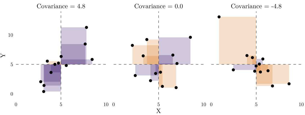
The covariance carries the units of \(x\) times the units of \(y\), the units of a rectangle’s area, so its size cannot be compared across pairs of variables. For example, the King County single family housing sales of 2025, the covariance of sale price and living area is about 517 million dollar-square-feet.
13.2 Pearson’s Correlation Coefficient
Dividing the covariance by both standard deviations, the Pearson correlation coefficient is the average product of the two z-scores:
\[r = \frac{s_{xy}}{s_x s_y} = \frac{1}{n-1}\sum_{i=1}^{n}\left(\frac{x_i - \bar{x}}{s_x}\right)\left(\frac{y_i - \bar{y}}{s_y}\right)\]
There is have no unit in correlation coefficients. It runs from \(-1\) to \(1\). \(r = 1\) or \(r = -1\) when every point lies on a straight line with a positive or negative slope; \(r = 0\) when there is no linear trend.
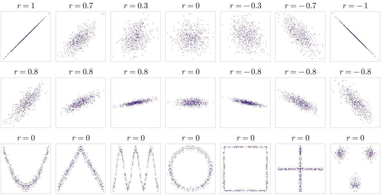
Notes about correlation: It shows linear relationship only. \(r\) measures how close the points are to a straight line. A non-linear curved relationship can have \(r = 0\). It is Symmetric. \(r\) for \((x, y)\) equals \(r\) for \((y, x)\), so it says nothing about which variable affects the other. Correlation is sensitive to outliers. A few extreme points can move \(r\) far in either direction.
Example 13.1 Boeing et al. (2023) compared Craigslist asking rents across 24 metropolitan areas with HUD’s Fair Market Rents, which determine Housing Choice Voucher payment limits. They found a moderate negative correlation between this rent gap and the local vacancy rate (\(r = -0.48\)), indicating that asking rents outpace voucher limits most sharply in tight housing markets.
13.2.1 Testing a Correlation
The sample correlation \(r\) estimates the population correlation \(\rho\). The test of \(H_0: \rho = 0\) uses
\[t = \frac{r\sqrt{n-2}}{\sqrt{1-r^2}}, \quad \text{df} = n - 2\]
In R, cor.test(x, y) reports \(t\), the p-value, and a confidence interval for \(\rho\). The test assumes independent pairs and, in small samples, roughly normal variables.
Example 13.2 In Example 13.1, \(t = -0.48\sqrt{22} / \sqrt{1 - 0.48^2} = -2.57\) with 22 df, so \(p = 0.018\), same with the paper’s “p < .05”. The 95% confidence interval for \(\rho\), computed as cor.test() does, runs from \(-0.74\) to \(-0.09\): with 24 areas, the sign is clear, but the strength is not.
13.3 Spearman’s Rank Correlation
Spearman’s rank correlation \(r_s\) is Pearson’s \(r\) computed on ranks: each \(x_i\) is replaced by its rank among the \(x\) values, and each \(y_i\) by its rank among the \(y\) values. Without ties,
\[r_s = 1 - \frac{6\sum_{i=1}^{n} d_i^2}{n(n^2-1)}\]
where \(d_i\) is the difference between the two ranks of case \(i\). \(r_s = 1\) whenever \(y\) always rises with \(x\), along a straight line or a curve, so \(r_s\) measures a monotonic relationship. A rank does not depend on how far out an extreme value is, so \(r_s\) suits skewed variables, outliers, and ordinal variables.
In Figure 13.3:
- Steeper. Twice the spread in \(y\) doubles the covariance; \(r\) and \(r_s\) do not change.
- Outlier. One far case pulls \(r\) from \(0.89\) to \(-0.10\), \(r_s\) only to \(0.41\).
- Curved. Always rising: \(r_s = 1\), \(r = 0.83\).
- U-Shaped. \(r = r_s = 0\): neither measures a relationship that changes direction.
- Two Groups. But no relationship inside either group.
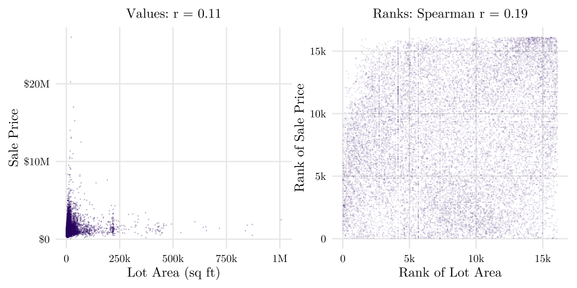
Example 13.3 Half of the King County lots are smaller than 7,511 square feet, and the largest is over a million. Of the 181 lots above 200,000 square feet, 178 are in unincorporated King County, mostly rural land that sells for ordinary prices. These few lots pull Pearson’s \(r\) between lot area and sale price down to 0.11; on ranks, they count no more than any other lot, and \(r_s = 0.19\).
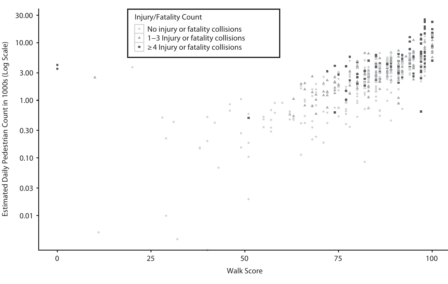
Example 13.4 Mooney et al. (2016) modeled pedestrian injuries at 532 New York City intersections, which needed the number of pedestrians at each. They estimated daily counts from nearby in-person counts and checked the estimates against Walk Score, a commercial walkability index from 0 to 100 based on the walking distances to nearby amenities such as grocery stores, schools, and parks (Walk Score methodology). The two correlated at Spearman \(r_s = 0.76\). Pedestrian counts span several orders of magnitude, so using Spearman’s works better than Pearson’s.
13.3.1 Kendall’s Tau
Instead of ranking all data points from 1 to \(n\) like Spearman’s correlation, Kendall’s tau (\(\tau\)) compares every possible pair of data points to see if they move in the same direction.
A pair is concordant if the case with the larger \(x\) also has the larger \(y\), and discordant if it has the smaller \(y\). With \(C\) concordant and \(D\) discordant pairs among the \(n(n-1)/2\) pairs, and no ties,
A pair is concordant if the observation with the larger (x) also has the larger (y), and discordant if the larger (x) has the smaller (y).
\[\tau = \frac{C - D}{n(n-1)/2}\]
Intuitively, this is the probability that a randomly chosen pair moves in the same direction minus the probability that it moves in opposite directions. In R, we use cor(x, y, method = "kendall").
13.4 Correlation Matrix
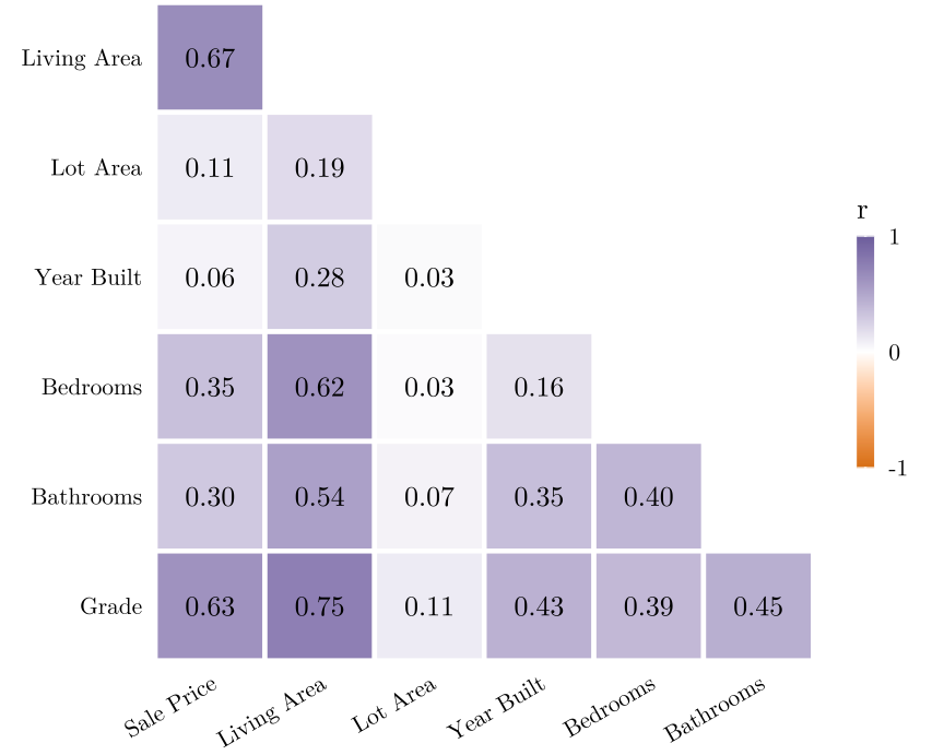
A correlation matrix lists the correlation of every pair among several variables. It is symmetric, with 1 on the diagonal, so half of it is enough.
13.5 Choosing a Measure
| Variables | Measure | Range | In R |
|---|---|---|---|
| Two numerical, linear relationship |
Pearson’s \(r\) | \(-1\) to \(1\) | cor(x, y) |
| Two numerical or ordinal, monotonic relationship |
Spearman’s \(r_s\); Kendall’s \(\tau\) | \(-1\) to \(1\) | cor(x, y, method = "spearman") or method = "kendall |
| Two or more ratings or measures of the same thing | Intraclass correlation (ICC); Cronbach’s \(\alpha\) | up to 1 | psych::ICC(d); psych::alpha(d) |
| Two categorical | Cramer’s V | 0 to 1 | from chisq.test() |
| A numerical and a categorical | \(\eta^2\) | 0 to 1 | from anova() |
| One variable across neighboring places | Moran’s I | about \(-1\) to \(1\) | spdep::moran.test() |
13.6 Reliability: ICC and Cronbach’s Alpha
Many measures in planning are judgments: a surveyor rates a house’s condition from the street or a reviewer scores a comprehensive plan. Others can be taken with more than one instrument, such as pedestrian counts in the field or on street-view images. When two raters score the same cases, or two instruments measure the same quantity, reliability asks whether the scores agree.
13.6.1 ICC
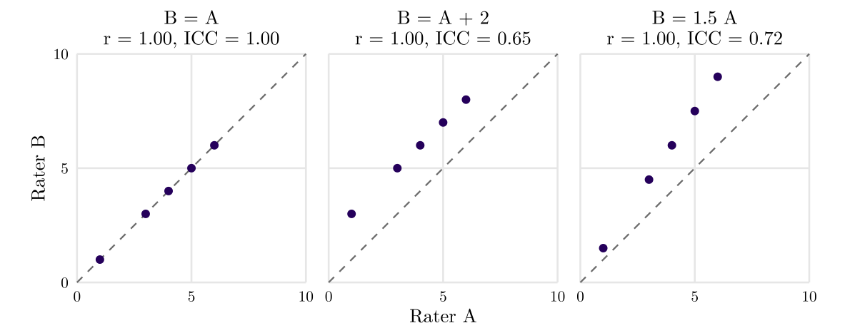
The intraclass correlation coefficient (ICC) is the share of the variance in the scores that comes from real differences among the cases rather than from the raters:
\[\text{ICC} = \frac{\sigma^2_{\text{cases}}}{\sigma^2_{\text{cases}} + \sigma^2_{\text{error}}}\]
where \(\sigma^2_{\text{cases}}\) is the variance of the cases’ true scores, how much the cases themselves differ, and \(\sigma^2_{\text{error}}\) the variance of the scores around each case’s true score, how much the raters miss it. The ICC is 1 when the raters agree exactly on every case and near 0 when the scores are mostly rater error.1
1 In R, psych::ICC(d), with one column per rater; read the ICC2 row.
A common reading calls an ICC above 0.8 almost perfect agreement and 0.6 to 0.8 substantial agreement (Tian, Musunuru and Ewing, 2020).
13.6.2 Cronbach’s Alpha
Cronbach’s alpha (\(\alpha\)) is the reliability of a score that adds \(k\) items (survey questions, raters, indicators) meant to measure one thing. It is used to check that the items move together before their sum is used as one measure:
\[\alpha = \frac{k}{k-1}\left(1 - \frac{\sum_{j=1}^{k} s_j^2}{s_T^2}\right)\]
where \(s_j^2\) is the variance of item \(j\) and \(s_T^2\) the variance of the total score. \(\alpha\) is 0 when the items are unrelated and 1 when they agree exactly.2
2 In R, psych::alpha(d), with one column per item.
When the items are raters scoring the same cases, both measure how well the raters agree. The ICC is the reliability of one rater’s score; \(\alpha\) is the reliability of the average of the \(k\) raters. Rater errors partly cancel in an average, so \(\alpha\) is higher: with an ICC of 0.5, the average of 4 raters has a reliability of 0.80 and the average of 10 raters 0.91.
Example 13.5 An expert panel rated 48 streetscape video clips on urban design qualities such as imageability and enclosure (Tian, Musunuru and Ewing, 2020). For imageability, the ICC was 0.49 and the panel’s Cronbach’s \(\alpha\) was 0.93: one panelist’s rating is a moderately reliable measure, and the panel’s average a highly reliable one.
Ewing et al. (2016) counted pedestrians on 588 New York City block faces in the field and again on Google Street View images, with \(\alpha = 0.864\) between the two counts. For Bing StreetSide images of 169 block faces, \(\alpha = 0.470\), below the 0.70 that some researchers require before they use a measure.
13.7 Correlation and Causation
A cause is usually required to come before its effect, to be associated with it, and to leave no other plausible explanation of the association (Shadish et al. 2001). A correlation shows only the second condition. An association between \(x\) and \(y\) can also come from:
- Chance. Among many pairs of variables, some correlate by luck.
- Reverse causation. \(y\) affects \(x\) instead of \(x\) affects \(y\).
- Confounding. A third variable, a confounder, affects both \(x\) and \(y\).
- Selection. The cases in the data were chosen by a variable that both \(x\) and \(y\) affect.

A test can say that an association is unlikely to be due to chance. It cannot say which of the other explanations produced it; that depends on how the data were produced.
For more than half a century, statisticians left causal questions out of statistics, on the view that data can show an association but not causality. The exception is the fully controlled experiment: when the researcher assigns \(x\) at random and treats the cases alike in every other way, a difference in \(y\) can be claimed as an effect of \(x\) (Pearl and Mackenzie 2018).
Example 13.6 In New York City, census tracts in historic districts have more educated and higher-income residents than other tracts: in 2010, more than 90% of their residents held a college degree, against 33% elsewhere (McCabe and Ellen 2016).
- Designation of historic districts may raise a neighborhood’s status (causation)
- Higher-income newcomers may be the ones who campaign for designation (reverse causation)
- Old, distinctive housing near the downtown may draw both designation of historic districts and higher-income residents (confounding)
The tracts later designated already had more college-educated residents in 1970, so part of the gap came before designation. Then, the authors compare each tract:
- with itself before and after designation (holding fixed its housing stock and location)
- with nearby tracts in the same decade (holding fixed local trends)
- with its own trend before designation (allowing for tracts that were already rising)
What remains is a rise of about 6% in average household income after designation.
13.8 Correlations of Aggregates
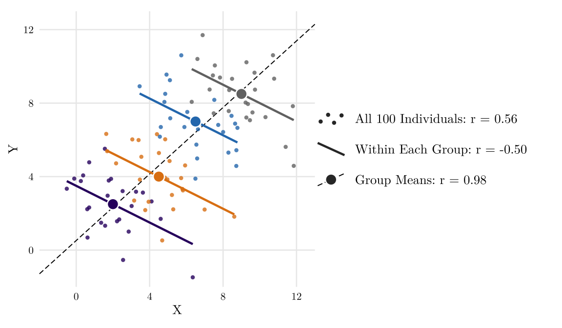
An ecological correlation is computed on group summaries, such as tract averages or city medians, rather than on individuals. Averaging removes the variation within groups, so an ecological correlation is usually stronger than the correlation among the individuals (Figure 13.10). Reading a relationship among individuals off it is the ecological fallacy (Gray et al. 2007).
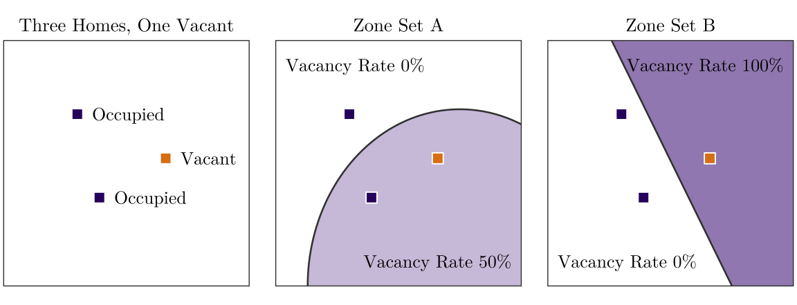
The same individuals grouped into larger or differently drawn units give different correlations. The problem exists in spatial data as well, known for the Modifiable Areal Unit Problem (MAUP).
13.9 Covariance and Correlation of RVs
\(s_{xy}\) and \(r\) describe a sample. For two random variables \(X\) and \(Y\), with expectations \(\mu_X\), \(\mu_Y\) and standard deviations \(\sigma_X\), \(\sigma_Y\), the same quantities come from their joint distribution, the probability of every pair of values. For discrete variables, the joint PMF is \(p(x, y) = P(X = x, Y = y)\).
The covariance of \(X\) and \(Y\) is the expected product of their deviations from their expectations:
\[\sigma_{XY} = \operatorname{Cov}(X, Y) = E[(X - \mu_X)(Y - \mu_Y)] = \sum_{x}\sum_{y} (x - \mu_X)(y - \mu_Y)\,p(x, y) = E[XY] - \mu_X \mu_Y\]
For continuous variables, a double integral over the joint density \(f(x, y)\) replaces the double sum. The population correlation is
\[\rho = \operatorname{Corr}(X, Y) = \frac{\operatorname{Cov}(X, Y)}{\sigma_X\,\sigma_Y}\]
\(s_{xy}\) and \(r\) estimate \(\sigma_{XY}\) and \(\rho\), as \(s^2\) estimates \(\sigma^2\).
- \(\operatorname{Cov}(X, X) = \operatorname{Var}(X)\).
- For constants \(a\), \(b\), \(c\), \(d\), \(\operatorname{Cov}(aX + b, cY + d) = ac\operatorname{Cov}(X, Y)\). A change of units changes the covariance but not \(\rho\), except for its sign when \(ac < 0\).
- \(\operatorname{Var}(X + Y) = \operatorname{Var}(X) + \operatorname{Var}(Y) + 2\operatorname{Cov}(X, Y)\). The rule for independent variables is the case \(\operatorname{Cov}(X, Y) = 0\).
- Independent variables have \(\operatorname{Cov}(X, Y) = 0\). The reverse fails: if \(X\) is symmetric around 0 and \(Y = X^2\), then \(\operatorname{Cov}(X, Y) = 0\), although \(Y\) depends entirely on \(X\) (the U shape in the bottom row of Figure 13.2).
Example 13.7 In Example 7.4, let \(X = 1\) in a year with a damaging earthquake (probability 0.05) and \(Y = 1\) in a year with a damaging landslide (0.03), and 0 otherwise. Suppose both happen in the same year with probability 0.02 (made up). For 0/1 variables, \(E[XY] = P(X = 1, Y = 1)\) and \(\sigma = \sqrt{p(1 - p)}\), so
\[\operatorname{Cov}(X, Y) = 0.02 - 0.05 \times 0.03 = 0.0185, \qquad \rho = \frac{0.0185}{\sqrt{0.05 \times 0.95}\,\sqrt{0.03 \times 0.97}} = 0.50\]
Independent hazards have \(P(X = 1, Y = 1) = 0.05 \times 0.03 = 0.0015\) and \(\rho = 0\).