11 Hypothesis Testing
No number of sightings of white swans can prove the theory that all swans are white. The sight of just one black swan can falsify it.
after Karl Popper
They are probably true, and probably not…
- Homes bought on a full moon gain value faster.
- Rents in Seattle rise in the years the Seahawks make the playoffs.
- My cat
 knows which block in Hong Kong will gentrify next.
11.1 The Scientific Method
The scientific method is a cycle of three stages (Gray et al. 2007), and a study can enter it at any stage1:
1 Research design is not a core topic of this course; see URBAN 512 or URBAN 591.
- Theories, hunches, and hypotheses. A theory is a general explanation of why things happen across many settings; it ties several hypotheses together, such as the bid-rent theory of how land values fall with distance from a center. A hunch is a less formal idea or guess that may later be refined into a theory. A hypothesis is a specific prediction that follows from a theory or a hunch.
- Observation and testing. Data are collected to check a theory or a hunch, or to build a new generalization from what is observed.
- Conclusions, or research findings. A supported hypothesis verifies the theory in one more setting; an unsupported one disconfirms it there and may lead to reformulating it. Findings rarely prove or disprove a theory outright; more often they refine it by stating the conditions under which it holds, and the cycle starts again.

Backyard cottage study. After Seattle eased its rules for detached accessory dwelling units (DADUs) in 2019, the city issued 128 DADU permits that year and 511 in 2022. In September 2020 the city released pre-approved DADU plans, designs it had approved in advance, and said they “will shorten the permitting process by at least 2-6 weeks” (SDCI). Do they? The hypothesis: DADU permits that use a pre-approved plan spend fewer days in city review than permits with custom designs.

A hypothesis must be falsifiable: some possible observation must be able to show that it is wrong. “Pre-approved plans will improve permitting process” is not falsifiable, since almost any outcome can be called an improvement of some kind. “At least 2-6 weeks faster” is falsifiable: permit records could show it wrong. The philosopher Karl Popper argued that this is what separates science from other claims. Observations can never prove a general hypothesis true (recall induction); a hypothesis earns our trust by surviving serious attempts to prove it false.
11.1.1 From Question to Hypothesis
In a quantitative study, a hypothesis becomes testable if it can be restated in terms of data. SDCI’s (Seattle Department of Construction & Inspections) building permit records provide, for every permit, the days it spent in the city’s hands between a complete application and the end of plan review.
“Pre-approved plans speed up review” somehow can become a comparison of two averages:
- The days in city review for DADU permits that used a pre-approved plan
- The days in city review for DADU permits with custom designs
Here, the response variables, dependent variable, or outcome, is the days in city review. The explanatory variable, independent variable or features, is the type of plan.
A statistical test can say whether the difference we observed is large enough to say it is not a coincidence. But we need to know whether the plans caused the difference is a separate question about causal inference.
11.2 Hypotheses
Example 11.1 Paul, an octopus in Oberhausen, Germany, “predicted” football (or soccer) matches by eating first from one of two boxes of food, each marked with a team’s flag. At the 2010 World Cup he picked the winner of all 8 matches he was given (Channel 4 News). If he was guessing, each pick was right with probability 1/2:
\[P(\text{8 of 8} \mid \text{guessing}) = \left(\tfrac{1}{2}\right)^8 = \tfrac{1}{256} \approx 0.004\]
Guessing cannot explain 8 of 8 well, yet few people concluded that an octopus can foresee football (or soccer). A claim that contradicts everything else we know needs much stronger evidence (much stronger than an event with 0.004 probability happened).
A hypothesis test starts in a similar way: assume the dull, default and safe explanation, and give it up only when the data would be very surprising if that explanation were true.
The DADU study has a dull explanation too. Between 2021 and 2025:
| Plan | Permits | Mean days in city review |
|---|---|---|
| Pre-approved | 250 | 42 |
| Custom | 816 | 69 |
| Difference | 27 |
Perhaps the pre-approval/custom designs make no difference, and the 27 days come from many coincidences driven by unique characteristics of the individual projects.
- The null hypothesis \(H_0\) is the dull explanation: no effect, no difference, only chance. The plan makes no difference, so mean days in city review are the same for pre-approved and custom plans: \(\mu_{\text{pre}} = \mu_{\text{custom}}\).
- The alternative hypothesis \(H_1\), also written \(H_A\), is the claim: mean review times differ, \(\mu_{\text{pre}} \ne \mu_{\text{custom}}\). \(H_1\) usually represents the novel discovery a study aims to validate, bearing the entire burden of empirical proof.
Both hypotheses are about the population, not the sample: \(\mu_{\text{pre}}\) is the mean of the permit process, not the 42 days and 69 days we have.
\(H_0\) always contains the equality, which makes it specific. In contrast, \(H_1\) contains an inequality (\(>\), \(<\), or \(\neq\)), such as stating that pre-approved plans are faster. Because “faster” is a vague, infinite range (is it faster by 1 day, 27 days, or 50 days?), \(H_1\) provides no specific point, and it is difficult to model.
This is why a test is built on \(H_0\). We choose to assume the exact world of \(H_0\) is true, and then check where our observation of 27-day gap lands on its curve. If our data lands so far out that the probability is extremely low, we can reject the \(H_0\), thereby supporting \(H_1\).

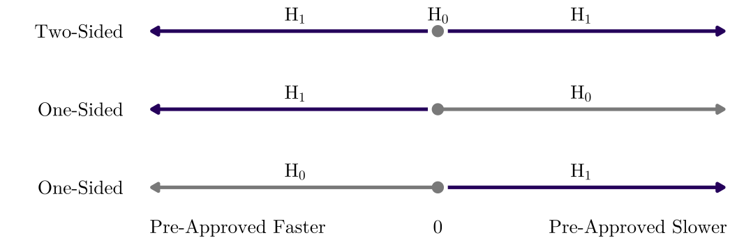
The alternative is two-sided when a difference in either direction counts, and one-sided when only one direction does. The city’s claim is one-sided, \(\mu_{\text{pre}} < \mu_{\text{custom}}\), but a pre-approved plan could also be slower, and only a two-sided test can detect that. The side is chosen before looking at the data; two-sided is the usual default.
11.3 The Logic of a Test
Under the hypothesis testing framework, almost every test follows the same steps:
- State \(H_0\) and \(H_1\), and choose a significance level \(\alpha\), commonly 0.05.
- Compute a test statistic: that measures how far the data are from what \(H_0\) predicts.
- Find the null distribution: the distribution of the test statistic if \(H_0\) were true.
- Compute the p-value: the probability, assuming \(H_0\) is true, of a test statistic at least as extreme as the one observed.
- If \(p \le \alpha\), reject \(H_0\); the result is statistically significant at level \(\alpha\). If \(p > \alpha\), fail to reject \(H_0\).
The logic resembles a criminal trial. The defendant is presumed innocent (\(H_0\)), and the verdict is guilty only if the evidence would be very surprising for an innocent person. A verdict of not guilty does not declare the defendant innocent. In the same way, failing to reject \(H_0\) does not show that \(H_0\) is true, only that the data are not strong enough to reject it (Diez et al. 2019).
11.3.1 Tests and Confidence Intervals
A two-sided test at level \(\alpha\) and a \((1 - \alpha)\) confidence interval are two readings of the same calculation: the test rejects \(H_0: \theta = \theta_0\) when \(\theta_0\) lies outside the confidence interval.
11.4 The Permutation Test
A permutation test builds the null distribution by reshuffling the group labels. It needs no assumption about the shape of the data and no large sample. It needs only that, under \(H_0\), the labels are exchangeable: each permit’s review time was as likely to carry one label as the other. That makes its null hypothesis stronger than equal means: under \(H_0\), the two groups’ whole distributions of review times are the same.
Example 11.2 From 2021 through 2025, Seattle issued the 1,066 DADU permits.
- The 250 with pre-approved plans spent on average 41.6 days in review
- The 816 with custom designs spent on average 68.9 days
If the type of plan carries no information about review time (\(H_0\)), the label (pre-approved or custom designs) landed on which permit was arbitrary. So we shuffle the labels at random, recompute the difference in means, and repeat plenty of times (4000 times in our case).
The shuffled differences run from \(-16.3\) to \(11.5\) days, and none comes near 27.3 in either direction, so \(p < 1/4{,}000\), and at \(\alpha = 0.05\) we reject \(H_0\).
We mention permutation test first because its logic is visible: the null distribution is something we construct and compare. Other tests in these two chapters replaces the shuffling process with a formula for the null distribution, faster but with assumptions.
11.5 Student’s t-Tests
The student’s t-tests replace the shuffling with a formula, using the t distribution as the null distribution. You may wonder why the name is “student’s t-test”, you can find the story about the origins of the Student’s t-test: William Sealy Gosset and his story at Guinness brewery in Dublin.
11.5.1 One Sample
To compare a sample mean with a fixed value \(\mu_0\), we compute the t statistic:
\[t = \frac{\bar{y} - \mu_0}{s / \sqrt{n}}, \qquad \text{df} = n - 1\]
Example 11.3 (Two-sided Test) In 2019, permits for a DADU alone (pre-approved and custom designs together) spent on average 72.4 days in city review. Did review take a different amount of time in 2025?
The 127 such permits issued in 2025 averaged 67.8 days, with a standard deviation of 26.8 (as given).
- \(H_0\): \(\mu_{2025} = 72.4\) days, the mean review time of 2025 is the same as in 2019.
- \(H_1\): \(\mu_{2025} \ne 72.4\) days.
We assume \(H_0\) is true, take 72.4 days as the fixed value, and compute the t statistic, which then follows the t distribution with 126 df:
\[t = (67.8 - 72.4) / (26.8 / \sqrt{127}) = -1.93\]
\(H_1\) is two-sided, so both tails count:
\[p = P(T \le -1.93 \text{ or } T \ge 1.93) = 2\,P(T \le -1.93)\]
R or SPSS gives \(p \approx 0.056 > 0.05\), so we fail to reject \(H_0\) at the 0.05 significance level.
Example 11.4 (One-sided Test) The pre-approved plans of 2020 were meant to shorten permitting. Did review take less time in 2025 than the 2019 average of 72.4 days? Now only one direction counts:
- \(H_0\): \(\mu_{2025} \ge 72.4\) days.
- \(H_1\): \(\mu_{2025} < 72.4\) days.
The test statistic is the same, \(t = -1.93\) with 126 df, but the p-value counts only the lower tail, \(p = P(T \le -1.93)\), half the two-sided p-value. So that \(p \approx 0.028 < 0.05\), and we reject \(H_0\).
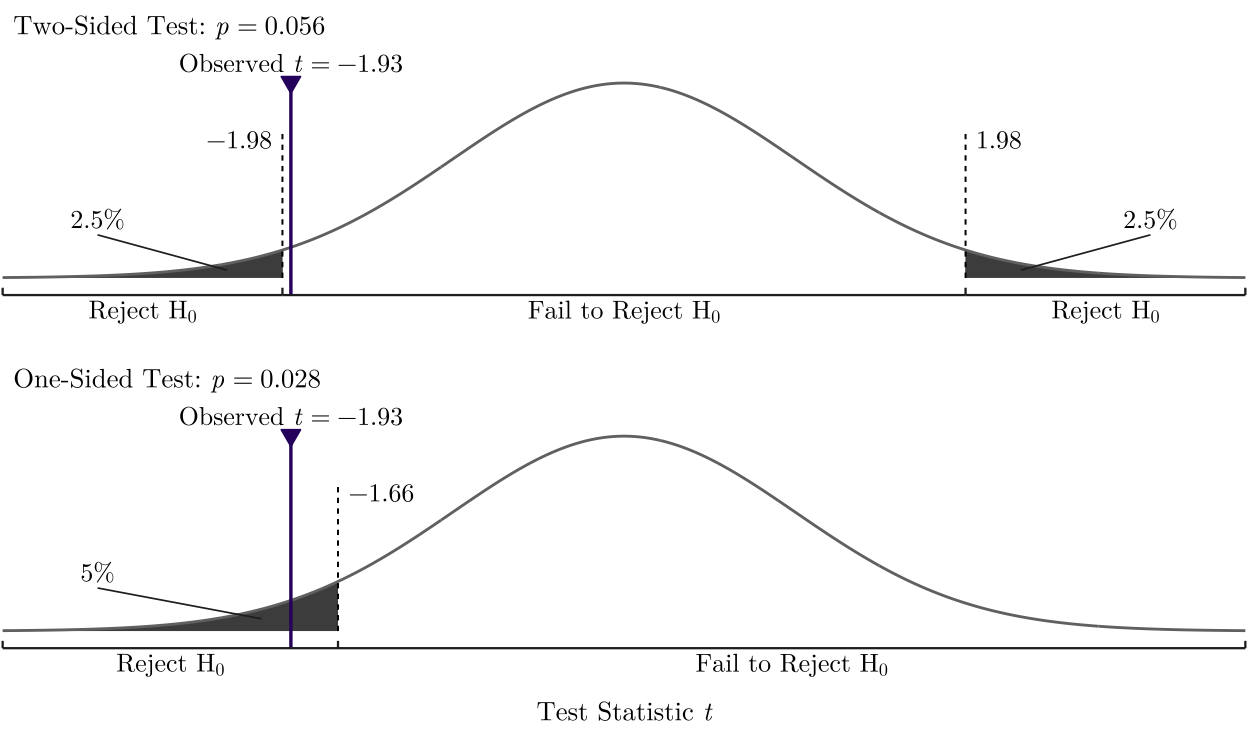
The two tests disagree at \(\alpha = 0.05\), and each test wrongly rejects a true \(H_0\) 5% of the time. The two-sided test splits the 5% between the tails (reject if \(|t| \ge 1.98\)); the one-sided test puts it all in the lower tail (reject if \(t \le -1.66\)) and cannot detect a slowdown.
11.5.2 Two Independent Samples
To compare the means of two independent groups, with sample means \(\bar{y}_1, \bar{y}_2\), standard deviations \(s_1, s_2\), and sizes \(n_1, n_2\):
\[t = \frac{\bar{y}_1 - \bar{y}_2}{\sqrt{s_1^2 / n_1 + s_2^2 / n_2}}\]
The denominator is the standard error of the difference (\(\bar{y}_1 - \bar{y}_2\)). This version, Welch’s t-test, estimates the two spreads separately, and we don’t assume two groups have same SD. It is R’s default (t.test() with var.equal = FALSE). Meanwhile, the classical pooled t-test (var.equal = TRUE) assumes the two groups have equal variances.
The t-test assumes that the observations are independent and that the sampling distribution of each mean is close to normal. Central limit theorem can guarantee it for moderate samples even when the data are skewed. However, if the data is heavy tails with a small sample size \(n\), we may need use the permutation test or the rank-sum test (below).
11.5.2.1 Why a t distribution
\(\bar{y}_1 - \bar{y}_2\) is close to normal (exactly normal for normal data, by the central limit theorem otherwise), with variance \(\sigma_1^2/n_1 + \sigma_2^2/n_2\). Divided by its true standard error, it would be a z-score. The formula divides by an estimate built from \(s_1\) and \(s_2\), which vary from sample to sample, so the statistic has the heavier tails of a t distribution. Its degrees of freedom depend on the version:
- Pooled t-test: \(n_1 + n_2 - 2\), the observations minus the two estimated means. With normal data and equal variances, the statistic follows this t distribution exactly.
- Welch’s t-test: only approximately t. Software computes the Welch-Satterthwaite degrees of freedom below; they lie between the smaller of \(n_1 - 1\) and \(n_2 - 1\), and \(n_1 + n_2 - 2\).
\[\nu_W = \frac{(s_1^2/n_1 + s_2^2/n_2)^2}{(s_1^2/n_1)^2/(n_1 - 1) + (s_2^2/n_2)^2/(n_2 - 1)}\]
11.5.3 Rank-Sum Test
A rank is a value’s position when all the values are sorted: 1 for the smallest, 2 for the next, and so on. You can imagine that it keeps only the order. A rank test runs on the ranks instead of the data values.
The Wilcoxon rank-sum test, also called the Mann-Whitney test, is the permutation test of Example 11.2 with ranks in place of the days; \(H_0\) is that neither group tends to have larger values.
Its statistic \(W\) counts, over every pair of one case from each group, how often the first group’s case is the larger (a tie counts as half), so \(W / (n_1 n_2)\) is the chance that a random case from the first group is larger than one from the second, about 0.5 under \(H_0\). It does not require normal sample means, and it works well for ordinal outcomes.
Example 11.5 In the 1,066 permits of Table 11.1, the median review took 33 days with a pre-approved plan and 57 days with a custom design. Over the \(816 \times 250 = 204{,}000\) pairs of one custom and one pre-approved permit, wilcox.test() gives
\[W = 151{,}240, \qquad \frac{W}{n_1 n_2} = \frac{151{,}240}{204{,}000} = 0.74, \qquad p < 0.001\]
Pick one custom and one pre-approved permit at random, and the custom one spent longer in city review 74% of the time.
11.5.4 Paired Samples
When the same units are measured twice, or the units come in matched pairs, compute the difference within each pair and run a one-sample t-test of the differences against 0. Pairing removes the variation between units, which is often most of the variation.
Example 11.6 In paired testing, two testers with similar qualifications but different race ask about the same advertised unit, and each records how many available units the agent tells them about. HUD’s Housing Discrimination Study 2012 ran such tests with Black and white renters in 28 metropolitan areas. Each test gives one pair of counts, and \(d\) is their difference: the units the white tester was told about minus the units the Black tester was told about. If the agent tells the white tester about 10 units and the Black tester about 8, \(d = 2\).
The data, from the 1,813 tests in which both testers met an agent:
- White testers were told about 1.83 units on average, Black testers about 1.63.
- The mean difference is \(\bar{d} = 1.83 - 1.63 = 0.20\) units.
- HUD reports its standard error, \(\operatorname{SE} = 0.05\). It equals \(s_d / \sqrt{n}\), so the 1,813 differences have an SD of about \(0.05 \times \sqrt{1{,}813} \approx 2.1\) units.
The hypotheses are about \(\mu_d\), the mean of \(d\) over all such tests:
- \(H_0\): \(\mu_d = 0\), agents tell Black and white renters about the same number of units on average.
- \(H_1\): \(\mu_d \ne 0\).
\[t = \frac{\bar{d}}{\operatorname{SE}} = \frac{0.20}{0.05} = 4.0, \qquad \text{df} = 1{,}812\]
Black renters were told about fewer units than white renters asking about the same unit, and a gap this large is very unlikely to be chance (\(p < 0.001\)).
11.6 Tests for Proportions
11.6.1 One Sample
To compare a sample share \(\hat{p}\) with a fixed value \(p_0\), we compute the z statistic. Under \(H_0\) the share is \(p_0\), so the standard error uses \(p_0\), not \(\hat{p}\):
\[z = \frac{\hat{p} - p_0}{\sqrt{p_0 (1 - p_0) / n}}\]
This is a Z-statistic because we use the theoretical SE based on the null hypothesis \(p_0\), rather than an estimated SE based on the sample.
The normal curve needs \(n p_0 \ge 10\) and \(n (1 - p_0) \ge 10\), ensuring a large enough sample (expecting at least 10 successes and 10 failures) to safely use the normal distribution for calculating the p-value. For a smaller sample, such as Paul’s 8 picks (Example 11.1), the p-value counts the possible outcomes exactly.
Example 11.7 Seattle’s 2024 ADU Annual Report counts 476 accessory dwelling unit permits in 2020, 246 of them for detached units (51.7%). Were detached and attached units equally common?
- \(H_0\): \(p = 0.5\), the share of detached units is one half.
- \(H_1\): \(p \ne 0.5\).
\[z = \frac{0.517 - 0.5}{\sqrt{0.5 \times 0.5 / 476}} = \frac{0.0168}{0.0229} = 0.73, \qquad p = 0.46\]
\(p = 0.46 > 0.05\), so we fail to reject \(H_0\) at the 0.05 significance level.
11.6.2 Two Independent Samples
For a share in two independent groups, the test of \(H_0: p_1 = p_2\) uses the pooled share \(\hat{p}\) of both groups combined. Each case is a 0/1 (Bernoulli) variable, whose SD is set by its share, \(\sqrt{p(1-p)}\), so under \(H_0\) the two groups have one common share and one common SD. The two shares are independent, so their variances, \(p(1-p)/n_1\) and \(p(1-p)/n_2\), add:
\[z = \frac{\hat{p}_1 - \hat{p}_2}{\sqrt{\hat{p}\,(1 - \hat{p})\,(1/n_1 + 1/n_2)}}\]
Example 11.8 Of the 1,066 permits of Table 11.1, 190 of 250 with a pre-approved plan (76.0%) and 310 of 816 with a custom design (38.0%) were issued within 90 days of a complete application.
- \(H_0\): \(p_{\text{pre}} = p_{\text{custom}}\), the share issued within 90 days is the same for both plans.
- \(H_1\): \(p_{\text{pre}} \ne p_{\text{custom}}\).
The pooled share is \(500 / 1{,}066 = 0.469\).
\[z = \frac{0.760 - 0.380}{\sqrt{0.469 \times 0.531 \times (1/250 + 1/816)}} = \frac{0.380}{0.0361} = 10.5\]
\(p < 0.001\), so we reject \(H_0\) at the 0.05 significance level.
11.7 Reading a Test Result
11.7.1 p-Value
A p-value is the probability of data like the data we observed if \(H_0\) is true \(P(\text{data} \mid H_0)\). It is not the probability that \(H_0\) is true given our data. Some common mistakes:
- A p-value is not the probability that \(H_0\) is true. \(P(\text{data} \mid H_0) \ne P(H_0 \mid \text{data})\).
- A p-value is not an effect size. With 200,000 households in each of two areas, cost-burden rates of 30.0% and 30.5% differ with \(p < 0.001\). The difference is statistically significant, but it doesn’t mean the difference is large.
- The threshold should not be treated as a cliff. \(p = 0.049\) and \(p = 0.051\) are practically the same evidence. Yet many studies report only whether \(p < 0.05\). Partly in response, the American Statistical Association issued in 2016 its first statement on a specific statistical practice: scientific conclusions and policy decisions should not rest only on whether a p-value passes a threshold (Wasserstein and Lazar 2016).
- A large p-value is not evidence of no effect. “Not significant” means that these data cannot reject \(H_0\). The possible reason may only be that the sample size was small.
11.7.2 Two Ways to Be Wrong
A test can make two kinds of error:
| \(H_0\) is true | \(H_0\) is false | |
|---|---|---|
| Reject \(H_0\) | Type I error (probability \(\alpha\)) | Correct decision (probability = power) |
| Fail to reject \(H_0\) | Correct decision (probability \(1 - \alpha\)) | Type II error (probability \(\beta\)) |
| Total | \(\alpha + (1 - \alpha) = 1\) | \(\text{power} + \beta = 1\) |
Type I error, a false alarm: rejecting \(H_0\) when it is true, \(P(\text{reject } H_0 \mid H_0 \text{ is true}) = \alpha\). We set it ourselves, before the test: with \(\alpha = 0.05\), a test of a true \(H_0\) rejects it 5% of the time.
Type II error, a miss: failing to reject \(H_0\) when it is false, \(P(\text{fail to reject } H_0 \mid H_0 \text{ is false}) = \beta\). It cannot be set; it depends on how large the true effect is and how much data we have. Power, \(1 - \beta\), is the chance that the test detects a real effect of a given size.
| Case | \(H_0\) | \(H_1\) | Type I error | Type II error |
|---|---|---|---|---|
| Criminal trial | The defendant is innocent | Guilty | Convict an innocent person | Acquit a guilty person |
| Disease test (Example 7.5) | No disease | Disease | False positive: treat a healthy person | False negative: miss a sick person |
| Pre-approved plans (Table 11.1) | Same mean review time as custom plans | A different mean review time | Credit the plans with a speedup they do not deliver | A program that works looks unproven |
The two errors trade off: a smaller \(\alpha\) moves the cutoffs outward, giving fewer false alarms (T1) and more misses (T2). In practice, the way to lower \(\beta\) without raising \(\alpha\) is a larger sample, which narrows both curves and pulls the cutoffs in.
11.7.3 Power and Sample Size
Before collecting data, we can work out how large a sample a test needs. Power depends on how large the true difference is, so first choose \(\delta\), the smallest true difference worth detecting. For two groups of equal size, comparing means, the sample size per group is
\[n = \frac{2\,(z_{1-\alpha/2} + z_{1-\beta})^2\,\sigma^2}{\delta^2}\]
- \(\delta\) (delta): the true difference in means to detect, in the units of the outcome.
- \(\sigma\) (sigma): the SD of the outcome within each of the two groups being compared, the spread among cases in the same group (permits with the same kind of plan), assumed equal in the two groups. It comes from earlier data or a pilot study. If the two SDs differ, replace \(2\sigma^2\) with \(\sigma_1^2 + \sigma_2^2\).
- \(z_{1-\alpha/2}\): the test’s cutoff on the z scale, 1.96 for a two-sided test at \(\alpha = 0.05\). We use z instead of t because t relies on sample size we don’t know.
- \(z_{1-\beta}\): the z-value with probability \(1 - \beta\) below it, 0.84 for power 0.80.
- \(n\): the number of cases in each group.
Where the formula comes from, step by step (Figure 11.8):
- Standard error of the difference in means, with \(n\) cases per group: \(\operatorname{SE} = \sigma \sqrt{2/n}\).
- The test rejects \(H_0\) beyond the cutoff \(1.96 \times \operatorname{SE}\).
- For power 0.80, 80% of the differences under \(H_1\), centered at \(\delta\), must land beyond that cutoff, so the cutoff is also \(\delta - 0.84 \times \operatorname{SE}\).
- Set the two cutoffs equal and solve for \(n\):
\[1.96\,\operatorname{SE} = \delta - 0.84\,\operatorname{SE} \;\Longrightarrow\; \delta = (1.96 + 0.84)\,\sigma\sqrt{\frac{2}{n}} \;\Longrightarrow\; n = \frac{2\,(1.96 + 0.84)^2\,\sigma^2}{\delta^2}\]
So \(n\) grows with \(\sigma^2\), with a stricter \(\alpha\), and with a higher power, and shrinks with \(\delta^2\): halving \(\delta\) takes four times the sample.
Example 11.9 How many permits per group would a new study need to detect a 20-day difference in mean city review time, with power 0.80 at \(\alpha = 0.05\)?
Custom permits in Example 11.2 have an SD of about 66 days, so \(\sigma = 66\) and \(\delta = 20\):
\[n = \frac{2\,(1.96 + 0.84)^2 \times 66^2}{20^2} \approx 171 \text{ permits per group}\]
A 10-day difference needs four times as many, about 683 per group.