12 Chi-Square Tests and ANOVA
The difference between “significant” and “not significant” is not itself statistically significant.
Andrew Gelman and Hal Stern (2006)
12.1 Choosing a Test
The type of the outcome and the number of groups decide the usual test.
| Outcome | Compared across | Question | Test |
|---|---|---|---|
| Numerical | A benchmark | Does the mean differ from a value? | One-sample t-test |
| Numerical | 2 groups | Do the two means differ? | Two-sample (Welch) t-test |
| Numerical | Matched pairs | Does the mean difference differ from 0? | Paired t-test |
| Numerical | 3 or more groups | Do any of the means differ? | One-way ANOVA |
| Skewed numerical or ordinal | 2 groups | Does one group tend to have larger values? | Wilcoxon rank-sum (Mann-Whitney) test |
| Skewed numerical or ordinal | 3 or more groups | Do some groups tend to have larger values? | Kruskal-Wallis test |
| Binary | A benchmark | Does the proportion differ from a value? | One-sample proportion z-test |
| Binary | 2 groups | Do the two proportions differ? | Two-proportion z-test |
| Categorical | Categories of another variable | Are the two variables independent? | Chi-square test |
Each test pairs with a measure of how large the difference or association is:
- The difference in means or proportions, for the t- and z-tests.
- \(W / (n_1 n_2)\) for the rank-sum test.
- \(\eta^2\) for ANOVA.
- Cramer’s V for the chi-square test.
Everything below this point in this lecture will not be in the quiz.
12.2 Contingency Tables
Previously, we read a contingency table with row, column, and total percentages. In the following table, the plan may explain the speed, so the percentages run within plan: 76.0% of pre-approved and 38.0% of custom permits were issued within 90 days.
Run the other way, the same table says that custom plans are 62.0% of the permits issued within 90 days and 89.4% of the slower ones (506 of 566).
They are the conditional probabilities \(P(\text{within 90 days} \mid \text{custom})\) and \(P(\text{custom} \mid \text{within 90 days})\), and only the first compares the two plans. Thus, before setting up a contingency table for a Chi-Square test, we must distinguish between the explanatory variable (the plan) and the response variable (the speed), ensuring our analysis relies on conditional probabilities conditioned on the explanatory variable.
| Within 90 days | Longer | Total | |
|---|---|---|---|
| Pre-approved | 190 (76.0%) | 60 (24.0%) | 250 (100.0%) |
| Custom | 310 (38.0%) | 506 (62.0%) | 816 (100.0%) |
| Total | 500 (46.9%) | 566 (53.1%) | 1,066 (100.0%) |
12.3 Chi-Square Test of Independence
The chi-square test asks whether the pattern in a contingency table could have come from chance. Two categorical variables are independent when the distribution of one is the same in every category of the other. Under independence, the expected count in the cell at row \(r\) and column \(c\) is
\[E_{rc} = \frac{(\text{row } r \text{ total}) \times (\text{column } c \text{ total})}{n}\]
and the test statistic adds up how far each observed count \(O\) is from its expected count \(E\):
\[\chi^2 = \sum_{\text{cells}} \frac{(O - E)^2}{E}, \qquad \text{df} = (\text{rows} - 1) \times (\text{columns} - 1)\]
Each term is squared, so \(\chi^2 \ge 0\), and a cell with more or with fewer cases than expected makes it larger either way. A \(\chi^2\) near 0 fits independence; a larger \(\chi^2\) is a evidence against independence. The test therefore rejects in the upper tail only.
Example 12.1 In Table 12.2, the expected count of pre-approved permits issued within 90 days is \(250 \times 500 / 1{,}066 = 117.3\), against 190 observed, so that cell contributes \((190 - 117.3)^2 / 117.3 = 45.1\).
The other three cells contribute 39.9, 13.8, and 12.2, so \(\chi^2 = 111.0\) with 1 df. The value that cuts off the top 5% of the chi-square distribution with 1 df is 3.84, and the p-value is below 0.0011: plan and speed are not independent.
1 The p-value can be found using pchisq(111.0, df = 1, lower.tail = FALSE) in R.
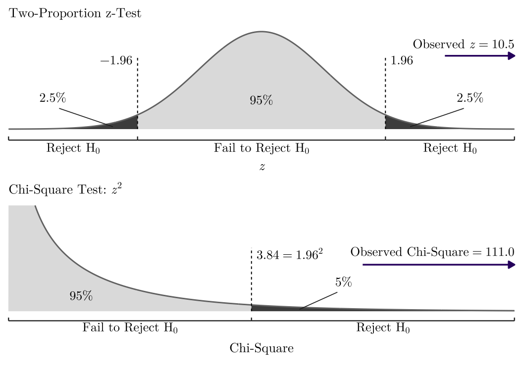
More often, we will use the chisq.test() in R directly. It applies a continuity correction to 2 by 2 tables by default and reports 109.5 for this table; chisq.test(x, correct = FALSE) reproduces 111.0. The correction makes the test slightly more conservative.
12.3.1 Cramer’s V
The chi-square statistic grows with the sample size and it tells us nothing about the strength of the association. A measure of strength that does not depend on \(n\) is Cramer’s V:
\[V = \sqrt{\frac{\chi^2}{n \times \min(\text{rows} - 1, \text{columns} - 1)}}\]
which runs from 0 (independence) to 1. Here \(V = \sqrt{111.0 / 1{,}066} = 0.32\). To see which cells drive the result, look at the standardized residuals of the cells; values beyond about \(\pm 2\) mark cells that differ from independence. The test assumes independent observations and an expected count of at least 5 in every cell. Also, it only says that the rows and columns are associated.
Example 12.2 Seattle’s 2024 ADU Annual Report counts the accessory dwelling unit (ADU) permits issued each year, split into attached and detached units. The 2019 reform took effect in August 2019, so 2018 and 2020 are the full years before and after it. Did the mix of the two types change?
| Attached | Detached | Total | |
|---|---|---|---|
| 2018 | 126 (51.4%) | 119 (48.6%) | 245 (100.0%) |
| 2020 | 230 (48.3%) | 246 (51.7%) | 476 (100.0%) |
| Total | 356 (49.4%) | 365 (50.6%) | 721 (100.0%) |
The expected count of attached units in 2018 is \(245 \times 356 / 721 = 120.97\), against 126 observed, so that cell contributes \((126 - 120.97)^2 / 120.97 = 0.209\). The other three cells contribute 0.204, 0.108, and 0.105.
So \(\chi^2 = 0.63\) with 1 df, and \(p = 0.43\). The total nearly doubled, from 245 to 476 permits, but the detached share moved only from 48.6% to 51.7%, a change the test cannot tell apart from chance.
12.4 Analysis of Variance (ANOVA)
With three or more groups, running a t-test for every pair runs into multiple comparisons (section below). Analysis of variance (ANOVA) asks whether there is any difference among the group means. In one-way ANOVA, we only consider one exploratory variable (one way of grouping): write \(y_{gi}\) for observation \(i\) in group \(g\), \(\bar{y}_g\) for the mean of group \(g\), \(\bar{y}\) for the overall mean, \(k\) for the number of groups, \(n_g\) for the size of group \(g\), and \(n\) for the total number of observations. ANOVA splits the total sum of square deviations into a part between the group means and a part within the groups:
\[\underbrace{\sum_{g=1}^{k}\sum_{i=1}^{n_g}(y_{gi}-\bar{y})^2}_{\text{total}} = \underbrace{\sum_{g=1}^{k} n_g(\bar{y}_g - \bar{y})^2}_{\text{between groups}} + \underbrace{\sum_{g=1}^{k}\sum_{i=1}^{n_g}(y_{gi}-\bar{y}_g)^2}_{\text{within groups}}\]
The F-statistic compares the two parts, each divided by its degrees of freedom (\(k - 1\) and \(n - k\)):
\[F = \frac{\text{between groups} / (k - 1)}{\text{within groups} / (n - k)}\]
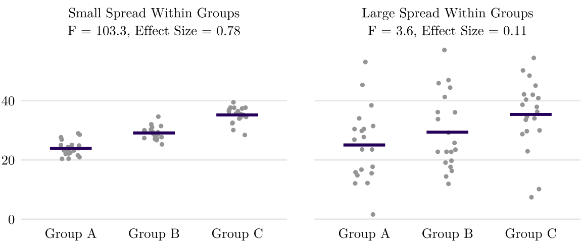
Under \(H_0\) that all \(k\) group means are equal. The \(F\) distribution is a ratio of two independent chi-square variables, each divided by its degrees of freedom. In ANOVA, a larger \(F\) statistic indicates that the between-group variance substantially exceeds the within-group variance, providing stronger evidence against equal group means (\(H_0\)).
ANOVA assumes:
- Independence: the observations are independent, within and across groups. Repeated measures of the same unit, or cases clustered in one place (neighborhoods of the same city) will break it.
- Normality: \(y\) is roughly normal within each group; check a histogram or Q-Q plot of the distances to the group means, \(y_{gi} - \bar{y}_g\). The central limit theorem covers moderate skew in moderate groups. With small groups and long tails or outliers, use the Kruskal-Wallis test.
- Equal variances: every group has the same variance \(\sigma^2\). It matters most when the group sizes differ. A rule of thumb: the largest group SD is less than twice the smallest. When the group variances differ, Welch’s version of the test drops the equal-variance assumption.
We mention that a significant test result cannot tell us the size of effect. The proportion of total variation explained by group differences, \(\eta^2 = \text{between} / \text{total}\), measures the overall effect size. In contrast, a significant \(F\)-test indicates only that at least two of the \(k\) group means differ.
Example 12.3 Did the time in city review change from year to year? The DADU permits issued from 2021 to 2025 (251, 249, 206, 233, and 127 permits) averaged 75.2, 67.8, 50.8, 50.6, and 67.8 days.
- \(H_0\): \(\mu_{2021} = \mu_{2022} = \dots = \mu_{2025}\).
- \(H_1\): at least two of the means differ.
\[F = 7.9, \quad \text{df} = (4, 1061), \quad p < 0.001, \quad \eta^2 = 0.029\]
The group SDs run from 99.9 days in 2021 down to 26.8 in 2025, far more than twice; Welch’s version gives \(F = 13.8\) with 4 and 502 df, \(p < 0.001\). The year does matter, but it accounts for about 3% of the variation in review time.
12.4.1 Kruskal-Wallis Test
The Kruskal-Wallis test is one-way ANOVA on ranks, for long tails or small sample sizes, or an ordinal outcome. Like the rank-sum test for two groups, it ranks all \(n\) cases together, from 1 for the smallest to \(n\) for the largest. Under \(H_0\), no group tends to have larger values. In R, we use kruskal.test().
Example 12.4 For the 1,066 permits of Example 12.3, the mean rank is \(533.5\):
| 2021 | 2022 | 2023 | 2024 | 2025 | |
|---|---|---|---|---|---|
| Mean days | 75.2 | 67.8 | 50.8 | 50.6 | 67.8 |
| Mean rank | 615.2 | 535.4 | 438.9 | 453.4 | 668.7 |
We can get the H statistic, \(H = 77.4\) with 4 df, \(p < 0.001\). 2021 has the highest mean but 2025 the highest mean rank: a few very long reviews in 2021 raise its mean but not its mean rank.
12.4.2 Beyond One-Way ANOVA
A one-way ANOVA compares groups formed by one categorical variable. But we have more designs, even though they are not widely used in urban planning:
- Two-way ANOVA: two grouping variables at once, such as plan and year, with a main effect for each and their interaction, whether the difference between plans changes from year to year.
- Repeated-measures ANOVA: the same units measured under every condition, such as the same neighborhoods in several years; it extends the paired t-test to more than two conditions.
- ANCOVA (analysis of covariance): group means compared after adjusting for a numerical variable, such as lot size.
- MANOVA (multivariate ANOVA): several outcomes compared at once.
12.5 Multiple Comparisons
A significant \(F\) says that some group means differ, not which ones. The natural next step compares every pair of groups, \(k(k-1)/2\) tests for \(k\) groups: 3 for three groups, 10 for the five years of Example 12.3. Each of them can make a Type I error.
If we run \(m\) hypothesis tests each at \(\alpha = 0.05\), on average \(0.05\times m\) of them make a Type I error. For independent tests, the probability of committing at least one Type I error is \(1 - 0.95^m\), which reaches 40% for 10 tests.
Example 12.5 We draw five groups, A to E, of 20 cases each from one normal distribution (mean 50, SD 10), so the five population means are equal and every \(H_0\) is true.
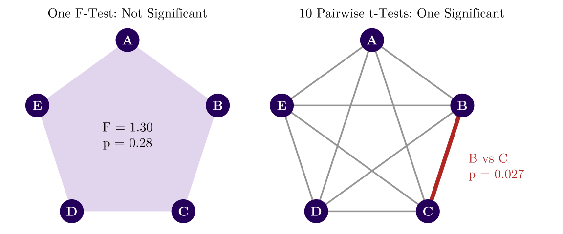
The ANOVA’s single \(F\)-test is not significant (\(F = 1.30\), \(p = 0.28\)). Yet one of the 10 pairwise t-tests is: B vs C, \(p = 0.027\); the other nine have \(p\) from 0.17 to 0.88.
A multiple-comparison correction adjusts the p-values of a family of tests so that the chance of even one Type I error in the whole family stays at or below \(\alpha\). Each test is then decided by its adjusted p-value.
- Bonferroni: multiply each p-value by \(m\) (capped at 1), the same as testing each at \(\alpha / m\).
- Holm: sort the p-values from smallest to largest, then multiply the smallest by \(m\), the next by \(m - 1\), and so on down to the largest, by 1; an adjusted p-value is never smaller than the one before it. Holm rejects at least as often as Bonferroni and is R’s default.
- Tukey’s method (
TukeyHSD()in R): specifically designed for comparing every pair of means after an ANOVA (assuming equal variances).
The ANOVA’s \(F\)-test, like a chi-square test of a whole table, is a single test and needs no correction; the pairwise comparisons after it are the family that does need multiple-comparison correction.
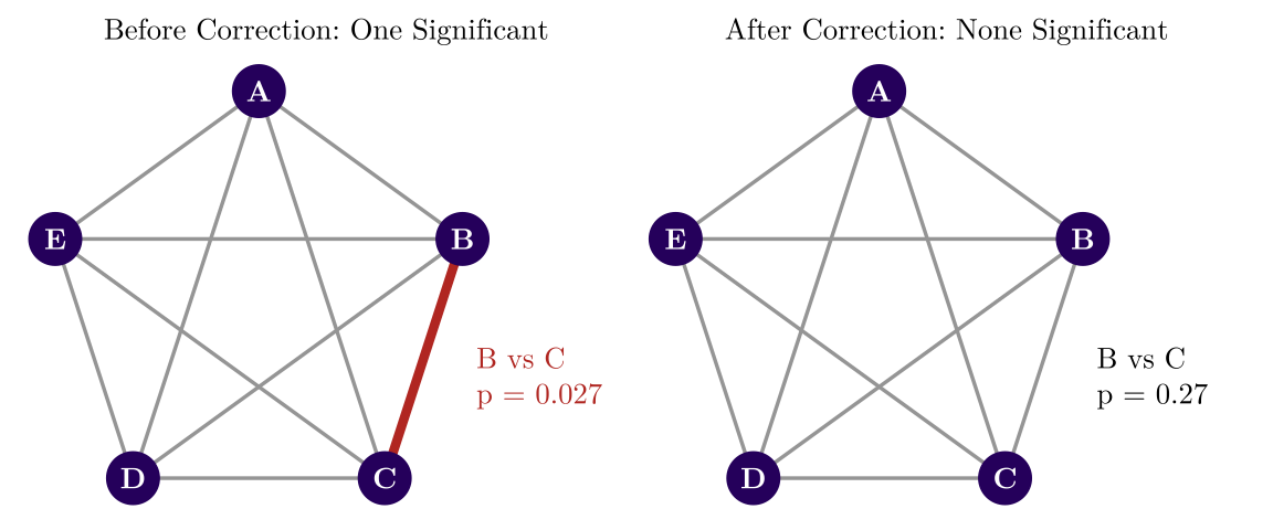
Example 12.6 Back to the 10 pairwise t-tests of Example 12.5, so \(m = 10\).
- Bonferroni multiplies every p-value by 10, and B vs C goes from 0.027 to \(10 \times 0.027 = 0.27\).
- Holm sorts the p-values: B vs C has the smallest, so it is also multiplied by 10, and the next, 0.17, is multiplied by 9 and capped at 1.
- Tukey’s method gives 0.17 for B vs C.
After any of the three corrections no pair is significant: the one Type I error is gone.
| Follow-up | R |
|---|---|
| Pairwise Means after ANOVA | pairwise.t.test() TukeyHSD() (best when with same SD) |
| Groups after Kruskal-Wallis | pairwise.wilcox.test() |
| Proportions after chi-square | pairwise.prop.test() |
| Any list of p-values | p.adjust(p, "holm") |
TukeyHSD(), which uses Tukey’s method, apply Holm’s correction by default.